A Pos­sible Idle RZ The­ory By Time

Guide writ­ten by Hack­zzzzzz. Con­tri­bu­tions from the Amaz­ing Com­munity.

This guide is cur­rently un­der­go­ing change. Keep in mind, strategies may change.

Feel free to use the gloss­ary as needed.

Ori­gin­ally From [LONG POST] A Pos­sible Idle RZ The­ory By Time - Eval­u­at­ing the Ef­fect of Time for Im­ple­ment­ing Black Hole on RZ CT Pro­gres­sion

Re­vised From Eval­u­at­ing the Ef­fect of Time for Im­ple­ment­ing Black Hole on Rho Pro­gres­sion of RZ CT and Eval­u­at­ing the Ef­fect of Time for Im­ple­ment­ing Black Hole on Delta Pro­gres­sion of RZ CT

TLDR: If u are go­ing to full idle RZ CT, get an ap­prox­im­a­tion of how long the pub will be, con­vert it into in-game $t$, and mul­tiply by 60% or 0.6, then com­pare to a table of “good” black hole $t$ to use with throughout your pub. DO NOT use it in a semi-idle/​act­ive situ­ation.

Ab­stract #

Im­ple­ment­ing black hole at the cor­rect time is very es­sen­tial for pro­gres­sion of RZ $\rho$ and $\delta$, and hence $\tau$ at an ef­fi­cient way. Due to tech­no­lo­gical dif­fi­culties of my­self, sev­eral ma­jor as­sump­tions are made in the pro­cess to en­sure a fair com­par­ison between data sets, in­clud­ing the ef­fect of the vari­ables $c_1$, $c_2$, $w_1$, $w_2$, $w_3$, and $b$ re­main the same throughout the pub­lic­a­tion. After a series of cal­cu­la­tion, it will be prac­tical and ideal with black hole im­ple­men­ted at 60% of the pub­lic­a­tion.

Meth­od­o­logy #

A data set of $t$, $z$ and $z^{\prime }$ had been ob­tained and un­dergo the ma­nip­u­la­tion of $\dot{\rho }$ and $\dot{\delta }$ re­spect­ively via. the for­mula provided in game, i.e., $\dot{\rho }=(timeinterval)\ast \frac{t}{\frac{z}{2^b}+0.01}$ & $\dot{\delta }=(timeinterval)\ast z^{\prime b}$. Then, cu­mu­lat­ive $\rho /\delta$ up to an ar­bit­rary time, $t$, was ma­nip­u­lated by sum­ming up all $\dot{\rho }/\dot{\delta }$ up to the time $t$. Fi­nally, by fix­ing $\dot{\rho }/\dot{\delta }$ after time $t$, which mim­icked the ef­fect of im­ple­ment­ing black hole, cu­mu­lat­ive $\rho /\delta$ was ma­nip­u­lated by sum­ming up all $\dot{\rho }/\dot{\delta }$ from $t=0$ un­til the end of the pub­lic­a­tion.

Take an ex­ample of $t=900$ sim­u­la­tion, given $\dot{\delta }$ for­mula in the game, $\delta$ can be ma­nip­u­lated as

In real game, the for­mula had already been its most sim­pli­fied form as the power of $w_1$ and $w_2$ var­ies when pur­chased. In this sim­u­la­tion, the as­sump­tion of the ef­fect $w_1$ and $w_2$ to be the same throughout the pub­lic­a­tion had been made. After black hole was im­ple­men­ted at an ar­bit­rary time $a$, $z^{\prime }$ were fixed, for­mula for cu­mu­lat­ive $\delta$ could be sim­pli­fied as

Do note that $w_3$ be­haves the same as $w_2$ with a lar­ger in­ter­val of pur­chas­ing. It has been omit­ted in the above-shown for­mula due to the fact that this study was pre­pared be­fore the ef­fect of $w_3$ was fully in­ter­pret by my­self. Mean­while, $w_3$ has no ef­fect on $\rho$ pro­gres­sion, so not ac­count­ing $w_3$ base on the as­sump­tion and for­mula given in game will have no net ef­fect on $\rho$ pro­gres­sion.

Next, a pub­lic­a­tion data set had been sim­u­lated with the fol­low­ing set­tings: Given a pub­lic­a­tion that had the same levels of $w_1$ and $w_2$ throughout, the cu­mu­lat­ive $\rho /\delta$ at the end of the pub­lic­a­tion had been ma­nip­u­lated with black hole im­ple­men­ted at vary­ing $t$ to­wards the end of the pub­lic­a­tion. Then, the res­ult could be visu­al­ized and rep­res­en­ted by plot­ting a graph of cu­mu­lat­ive $\rho /\delta$ at the end of the pub­lic­a­tion against the time for im­ple­ment­ing the black hole.

In short, one should in­ter­pret the graphs as the fol­low­ing:

• $y$-axis is the max­imum $\rho /\delta$ (in ar­bit­rary unit) ob­tained at the end of the pub­lic­a­tion

• $x$-axis is the time, in $t$, when black hole is be­ing im­ple­men­ted

It is worth not­ing that $y$-axis for cu­mu­lat­ive $\rho$ and cu­mu­lat­ive $\delta$ are in ar­bit­rary units, and they de­vi­ate from the real res­ult by a lin­ear factor (af­fected by $c_1$, $c_2$, $w_1$, $w_2$, and $w_3$).

The above cal­cu­la­tions are all per­formed in Mi­crosoft Ex­cel with for­mula im­ple­men­ted in all data sets.

Res­ult #

Eval­u­at­ing the ef­fect of the time of im­ple­ment­ing black hole on $\rho$ & $\delta$ pro­gres­sion un­der con­stant $b$ #

4 dif­fer­ent data sets were tested with the sim­u­la­tion of $b=1.5$ and the res­ults were ob­tained, they were:

1. A pub­lic­a­tion at $t=40,000$ with time in­ter­val 1. Max­imum cu­mu­lat­ive $\rho$ res­ul­ted at $t=40,000$ if black hole is im­ple­men­ted at $t=18,047$ (45.1%; Graph 1a). Max­imum cu­mu­lat­ive $\delta$ res­ul­ted at $t=40,000$ if black hole is im­ple­men­ted at $t=14,304$ (35.8%; Graph 1b).

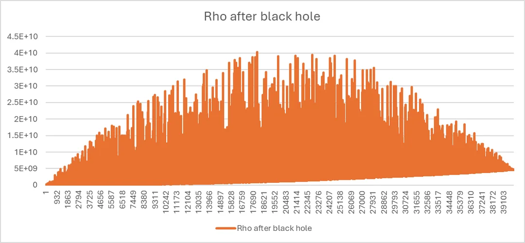
Graph 1a: a pub­lic­a­tion of $t=40,000$, with cu­mu­lat­ive $\rho$ plot­ted against time of im­ple­ment­ing black hole in lin­ear scale

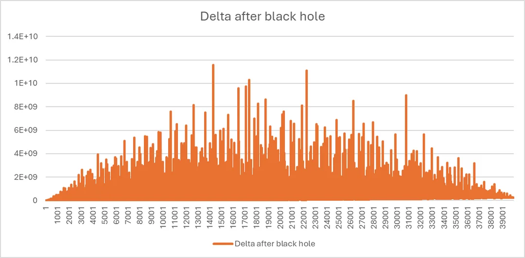
Graph 1b: a pub­lic­a­tion of $t=40,000$, with cu­mu­lat­ive $\delta$ plot­ted against time of im­ple­ment­ing black hole in lin­ear scale ($b=3$)

2. A pub­lic­a­tion at $t=900$ (i.e., a pub­lic­a­tion with 1 hour in real time) with time in­ter­val 0.01. Max­imum cu­mu­lat­ive $\rho$ res­ul­ted at $t=900$ if black hole is im­ple­men­ted at $t=466.56$ (51.8%; Graph 2a). Max­imum cu­mu­lat­ive $\delta$ res­ul­ted at t = 900 if black hole is im­ple­men­ted at t = 480.40 (53.3%; Graph 2b).

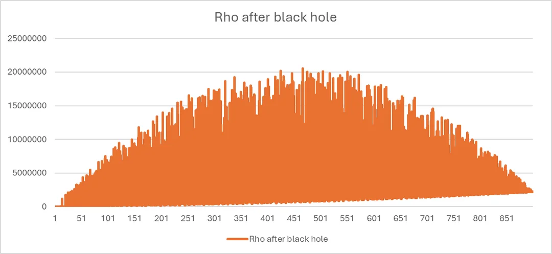
Graph 2a: a pub­lic­a­tion of $t=900$, with cu­mu­lat­ive $\rho$ plot­ted against time of im­ple­ment­ing black hole in lin­ear scale

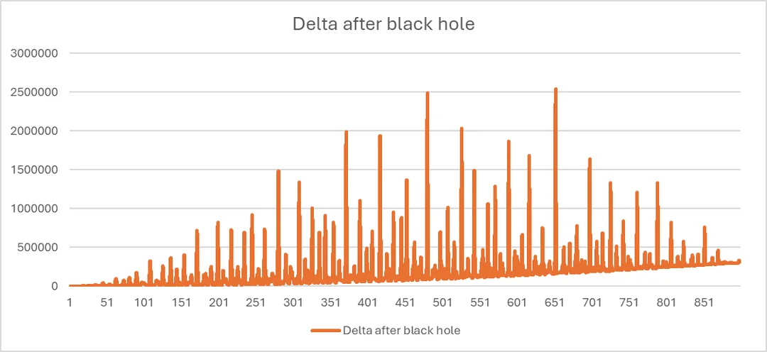
Graph 2b: a pub­lic­a­tion of $t=900$, with cu­mu­lat­ive $\delta$ plot­ted against time of im­ple­ment­ing black hole in lin­ear scale ($b=3$)

3. A pub­lic­a­tion at $t=1,800$ (i.e., a pub­lic­a­tion with 2 hours in real time) with time in­ter­val 0.01. Max­imum cu­mu­lat­ive $\rho$ res­ul­ted at $t=1,800$ if black hole is im­ple­men­ted at $t=957.5$ (53.2%; Graph 3a). Max­imum cu­mu­lat­ive $\delta$ res­ul­ted at $t=1,800$ if black hole is im­ple­men­ted at $t=652.21$ (36.2%; Graph 3b).

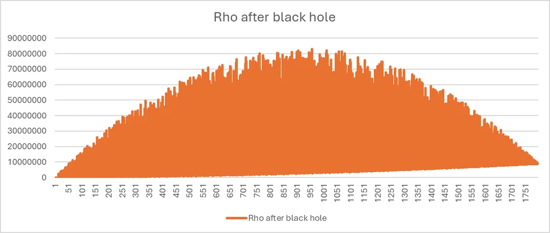
Graph 3a: a pub­lic­a­tion of $t=1,800$, with cu­mu­lat­ive $\rho$ plot­ted against time of im­ple­ment­ing black hole in lin­ear scale

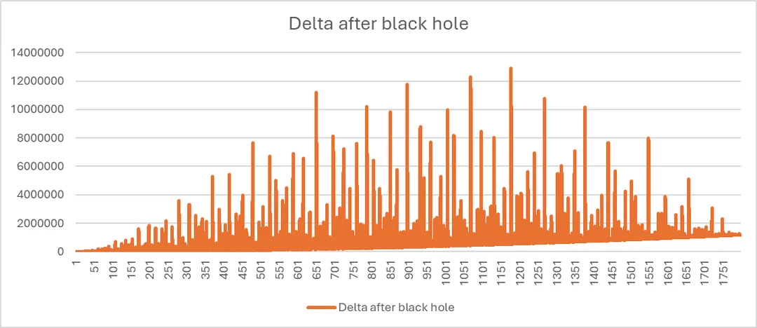
Graph 3b: a pub­lic­a­tion of $t=1,800$, with cu­mu­lat­ive $\delta$ plot­ted against time of im­ple­ment­ing black hole in lin­ear scale ($b=3$)

4. A pub­lic­a­tion at $t=1,500$ (i.e., a pub­lic­a­tion with 100 minutes in real time) with time in­ter­val 0.01. Max­imum cu­mu­lat­ive $\rho$ res­ul­ted at $t=1,500$ if black hole is im­ple­men­ted at $t=762.69$ (50.8%; Graph 4a). Max­imum cu­mu­lat­ive $\delta$ res­ul­ted at $t=1,500$ if black hole is im­ple­men­ted at $t=652.21$ (43.5%; Graph 4b).

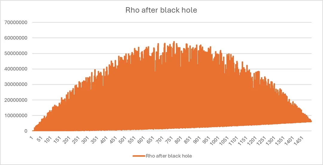
Graph 34: a pub­lic­a­tion of $t=1,500$, with cu­mu­lat­ive $\rho$ plot­ted against time of im­ple­ment­ing black hole in lin­ear scale

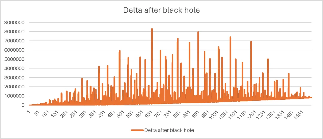
Graph 4b: a pub­lic­a­tion of $t=1,500$, with cu­mu­lat­ive $\delta$ plot­ted against time of im­ple­ment­ing black hole in lin­ear scale ($b=3$)

All 4 data sets showed sim­ilar res­ults that max­imum cu­mu­lat­ive $\rho$ was ob­tained at the end of the pub­lic­a­tion if black hole is im­ple­men­ted at 50% of the pub­lic­a­tion, while they showed dis­tinct res­ults that max­imum cu­mu­lat­ive $\delta$ was ob­tained at the end of the pub­lic­a­tion if black hole is im­ple­men­ted at dif­fer­ent time (de­pend on $z^{\prime }$ and $b$). No con­clu­sion can be drawn for $\delta$ pro­gres­sion.

Eval­u­at­ing the ef­fect of vary­ing $b$ on cu­mu­lat­ive $\rho$ & $\delta$ #

As $b$ has no ef­fect on $\dot{\rho }$ after black hole is im­ple­men­ted, it can be con­cluded that $b$ has no al­ter­a­tion on the res­ult on the time of im­ple­ment­ing black hole for max­imum cu­mu­lat­ive $\rho$ to be ob­tained based on the ma­jor as­sump­tion of con­stant ef­fect of $c_1$, $c_2$, $w_1$, $w_2$, and $w_3$ throughout the pub­lic­a­tion.

The 4 above-men­tioned data sets were re­peated with the sim­u­la­tion of $b=1.5$ (i.e., Level 3), $b=2$ (i.e., Level 4), $b=2.5$ (i.e., Level 5), and $b=3$ (i.e., Level 6). The res­ults were ob­tained and were

1. A pub­lic­a­tion at $t=40,000$ with time in­ter­val 1 (Graph 5).

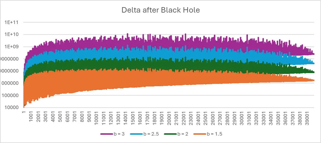
Graph 5: a pub­lic­a­tion of $t=40,000$, with cu­mu­lat­ive $\delta$ plot­ted against time of im­ple­ment­ing black hole in log scale

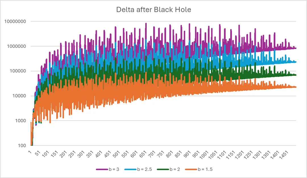
2. A pub­lic­a­tion at $t=900$ (i.e., a pub­lic­a­tion with 1 hour in real time) with time in­ter­val 0.01 (Graph 6).

Graph 6: a pub­lic­a­tion of $t=900$, with cu­mu­lat­ive $\delta$ plot­ted against time of im­ple­ment­ing black hole in log scale

3. A pub­lic­a­tion at $t=1,800$ (i.e., a pub­lic­a­tion with 2 hours in real time) with time in­ter­val 0.01 (Graph 7).

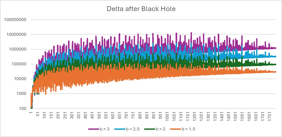
Graph 7: a pub­lic­a­tion of $t=1,800$, with cu­mu­lat­ive $\delta$ plot­ted against time of im­ple­ment­ing black hole in log scale

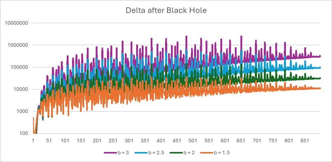
4. A pub­lic­a­tion at $t=1,500$ (i.e., a pub­lic­a­tion with 100 minutes in real time) with time in­ter­val 0.01 (Graph 8).

Graph 8: a pub­lic­a­tion of $t=1,500$, with cu­mu­lat­ive $\delta$ plot­ted against time of im­ple­ment­ing black hole in log scale

The res­ult can be sum­mar­ized as the fol­low­ing table:

Table: The time of im­ple­ment­ing black hole, $t$, and max­imum cu­mu­lat­ive $\delta$ ob­tained (Cu­mu­lat­ive $\delta$; in ar­bit­rary units) for 4 Data sets with vary­ing $b$

Con­clu­sion and Dis­cus­sion #

Con­clu­sion #

The above in­vest­ig­a­tions il­lus­trate the fact that im­ple­ment­ing black hole at dif­fer­ent times does af­fect the cu­mu­lat­ive $\rho$ ob­tained at the end of the pub­lic­a­tion, thus af­fect­ing the time re­quired for pub­lic­a­tion and ef­fi­ciency of gain­ing $\tau$ for growth. Sim­u­la­tion across dif­fer­ent data sets also demon­strates the con­sist­ency of im­ple­ment­ing black hole at 50% of the pub­lic­a­tion for op­tim­iz­a­tion, and the hy­po­thesis that the dur­a­tion of pub­lic­a­tion seems to be in­de­pend­ent to the ab­so­lute time of im­ple­ment­ing the black hole (only the re­l­at­ive dur­a­tion does).

Im­ple­ment­ing black hole at dif­fer­ent times does not con­sist­ently af­fect the cu­mu­lat­ive $\delta$ ob­tained at the end of the pub­lic­a­tion. Cal­cu­la­tions across dif­fer­ent data sets demon­strate fluc­tu­at­ing res­ult on the time im­ple­ment­ing the black hole. Graphs 5–8 re­veal a fact that the value of $b$ is a ma­jor factor af­fect­ing the time for im­ple­ment­ing black hole to ob­tain max­imum cu­mu­lat­ive $\delta$, which is dif­fer­ent from that by ma­nip­u­lat­ing cu­mu­lat­ive rho.

Eval­u­at­ing the Ef­fect of $c_1$, $c_2$, $w_1$, $w_2$, and $w_3$ #

The above sim­u­la­tions took on a ma­jor as­sump­tion of a pub­lic­a­tion that had the same levels of $c_1$, $c_2$, $w_1$, $w_2$, and $w_3$ throughout, which al­lowed the ma­nip­u­la­tion of cu­mu­lat­ive $\rho /\delta$ in a single in­de­pend­ent vari­able set­ting and hence val­id­ated the fair com­par­ison among in­de­pend­ent vari­ables. However, such as­sump­tion was prac­tic­ally im­possible dur­ing the ac­tual situ­ation. As the ef­fect of vari­ables on the cu­mu­lat­ive $\rho$ is com­plex and highly de­pend­ent on the act­ive­ness of player, it was also the­or­et­ic­ally chal­len­ging to sim­u­late the ex­act ef­fects on all avail­able data I had in my ex­cel. To eval­u­ate the gen­eral/​rough ef­fects of $c_1$, $c_2$, $w_1$, $w_2$, $w_3$, and $b$, I will ex­plore them in the view of the equa­tion of $\dot{\rho }$ and $\dot{\delta }$ in-game and in turn eval­u­ate the ef­fect of such on the graphs, hence provide a more re­fined hy­po­thesis.

1. The cost of pur­chas­ing $c_1$, $c_2$, $w_1$, $w_2$, $w_3$, and $b$ has no ef­fect on the graphs, as the graphs plot the cu­mu­lat­ive $\rho /\delta$, not the $\rho /\delta$ a player have at a spe­cific $t$.

2. The ef­fect of $c_1$, $c_2$, and $w_1$ will shift the graphs of cu­mu­lat­ive $\rho$ up­ward and right­ward at a non-lin­ear scale, as $\dot{\rho }$ dir­ectly de­pends on $c_1$, $c_2$, and $w_1$.

3. $c_1$ and $c_2$ has no ef­fect on the graphs of cu­mu­lat­ive $\delta$, as they have no re­la­tion­ship on $\dot{\delta }$.

4. The ef­fect of $w_1$, $w_2$, and $w_3$ will shift the graphs of cu­mu­lat­ive $\delta$ up­ward and right­ward at a non-lin­ear scale, as $\dot{\delta }$ dir­ectly de­pends on $w_1$, $w_2$, and $w_3$.

5. The ef­fect of $b$ will shift the graph of cu­mu­lat­ive $\rho$ up­ward at a non-lin­ear scale and cu­mu­lat­ive $\delta$ up­ward at an ex­po­nen­tial scale, as it dir­ectly in­flu­ences $\dot{\delta }$ in an ex­po­nen­tial man­ner and hence $\dot{\rho }$ in­dir­ectly.

6. The ef­fect of shortened time buy­ing the vari­ables will shift the graphs of cu­mu­lat­ive $\rho$ and $\delta$ left­ward at a non-lin­ear scale, as it al­lows an earlier growth for cu­mu­lat­ive $\rho$ and $\delta$ in a re­peat­able man­ner.

Over­all, pur­chas­ing $c_1$, $c_2$, $w_1$, $w_2$, $w_3$, and $b$ have an ef­fect of shift­ing graphs up­ward and slightly right­ward, in­dic­at­ing the im­ple­ment of black hole is pos­sible to be pushed back slightly for op­tim­iz­a­tion.

The above-men­tioned ef­fects were later veri­fied by the sim (with the most op­timal strategy im­ple­men­ted by brute-for­cing dif­fer­ent $t$ for im­ple­ment­ing black hole on a pub), which takes into the ac­count of the ef­fects of vari­able pur­chases (i.e., $c_1$, $c_2$, $w_1$, $w_2$, $w_3$, and $b$) and us­age of level chas­ing strategy (Us­ing a ra­tio of ap­prox­im­ately 4x in terms of levels for $c_1$ over $c_2$). The dur­a­tion of a pub­lic­a­tion, the time of im­ple­ment­ing black hole and their re­l­at­ive per­cent­age, $\frac{t_{bh}}{t_{pub}}$, has been cal­cu­lated and plot­ted as a graph of re­l­at­ive dur­a­tion against $\tau$ (Graph 9).

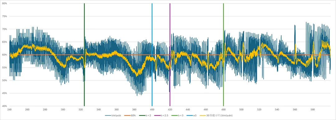
Graph 9: Re­l­at­ive time of im­ple­ment­ing black hole plot­ted against dif­fer­ent $\tau$, with or­ange ho­ri­zontal line as 60% line and yel­low plots as 30 mov­ing av­er­age for re­l­at­ive time

The plot sup­ports the con­sist­ency of im­ple­ment­ing black hole at 60% of the pub­lic­a­tion for achiev­ing a more ideal out­come by op­tim­iz­a­tion of cu­mu­lat­ive $\rho$. One point worth not­ing is that the re­l­at­ive dur­a­tion for black hole im­ple­ment­a­tion tem­por­ar­ily spiked up upon a $w_3$ and/​or $b$ up­grade, in­dic­at­ing a longer pub­lic­a­tion, and hence a later time for im­ple­ment­ing black hole.

Eval­u­at­ing the Ac­tual Time for Im­ple­ment­ing Black Hole #

Im­ple­ment­ing the black hole at the right time is es­sen­tial for $\rho /\tau$ growth since it fixes $z^{\prime }$ as well. However, the con­tinu­ity of the pub­lic­a­tion dur­a­tion does not have the same nature of the dis­crete­ness of the solu­tion for $z=0$, which may lead to sub­op­timal $z^{\prime }$ if the hy­po­thesis is strictly fol­lowed.

In re­sponse of this, there are also data from Dis­cord about $z=0$ with par­tic­u­larly higher $z^{\prime }$ as a list. One can con­sider se­lect­ively set­ting t with $z=0$ and high $z^{\prime }$ as the time of im­ple­ment­ing black hole in­stead of the the­or­et­ical val­ues ob­tained from the hy­po­thesis. From the graphs above, it can be ob­served that se­lect­ing a time for im­ple­ment­ing black hole that slightly de­vi­ates from the hy­po­thes­ized time min­im­ally af­fect the cu­mu­lat­ive $\rho /\delta$ ob­tained at the end of the pub­lic­a­tion.

Pro­pos­ing a Pos­sible New Idle Route for Com­ple­tion of RZ CT #

Base on the dis­cus­sion and all avail­able data we have at this mo­ment, it may be reas­on­able to pro­pose a new idle route of pub­lic­a­tion for com­ple­tion of RZ CT after e600 $\rho$ the gen­eral rout­ing will be as fol­low:

1. Take an es­tim­ate on the dur­a­tion of the up­com­ing pub­lic­a­tion wish to be idled. Cal­cu­late the hy­po­thes­ized time for im­ple­ment­ing black hole (i.e., 60% of your pub­lic­a­tion time. Do es­tim­ate a longer time if a $w_3$ and/​or $b$ up­grade is close to your pre­vi­ous pub­lic­a­tion point).

2. Set the time for im­ple­ment­ing black hole that is $z=0$ and has a high $z^{\prime }$ and is suf­fi­ciently close to the hy­po­thes­ized time cal­cu­lated from pre­vi­ous step.

3. Start play­ing the pub­lic­a­tion with auto­buy all (as miss­ing $c_1$ and $w_1$ pur­chases af­fect the pro­gress heav­ily if it is missed for a sig­ni­fic­ant por­tion of time).

4. When the black hole is im­ple­men­ted, con­tinue to auto­buy un­til the end of pub­lic­a­tion.

5. Re­peat the pro­gress if the next pub­lic­a­tion is also des­ig­nated to be idled.

Ac­know­ledge­ment #

Lastly, I would like to give a huge thanks to the fol­low­ing people/​group of people for as­sist­ing the veri­fic­a­tion of hy­po­thesis and fur­ther find­ings on RZ CT:

• Prop

  • For design­ing the RZ CT, provid­ing data for pro­cessing and veri­fy­ing the hy­po­thesis, and re­fin­ing on the ac­cur­acy of the hy­po­thesis.

• Hotab, Mathis S.

  • For design­ing the sim­u­la­tion for RZ CT and sug­gest­ing the concept of de­vi­at­ing from the­or­et­ical time and se­lect­ing $t$ with high $z^{\prime }$.

• in­valid.user_, Megam­inx

  • For sug­gest­ing the point of as­sess­ing the ef­fect of $b$ on cu­mu­lat­ive $\rho$ and $\delta$, and bring­ing up sev­eral points in dis­cus­sion sec­tion to in­vest­ig­ate with.

• Axiss, lll333, Black Seal, Mathis S., Megamin, Maimai

  • For will­ing to test my hy­po­thesis with their save and bring­ing up sev­eral points on my hy­po­thesis. (ofc, thanks Maimai for en­light­en­ing of RZyoyoyo lol)

• All other people

  • For provid­ing ex­per­i­mental data and provid­ing sup­port whenever I need them.