Visu­al­iz­ing Vari­able Power Throughout the Game

Guide writ­ten by spqcey. Con­tri­bu­tions from the Amaz­ing Com­munity.

Feel free to use the gloss­ary as needed.

Ini­tial Pub­lic­a­tion on Novem­ber 19, 2022

Some in­form­a­tion (with re­gards to top play­ers) may be in­ac­cur­ate

In­tro­duc­tion #

Let’s start by de­fin­ing which vari­ables we’re dis­cuss­ing. We will dis­cuss the main-game vari­ables, ($x-\xi$), NOT the up­grades bought in the­or­ies.

We can split the pro­gres­sion through the game into three sec­tions:

• From 0 to ee4310, this sec­tion in­cludes the un­lock­ing of all of the vari­ables, fin­ish­ing with the un­lock­ing of $\xi$ at ee791. It also in­cludes the pur­chase of $y$ power up­grades, of which we will dis­cuss more later.

• From ee9160 to ee47362, this is the range when we buy su­prem­acy up­grades known as “psi3” up­grades.

• Fi­nally, the fi­nal sec­tion is after ee47362, where we see the title of strongest vari­able change hands a few more times with a fi­nal change at ~ee70000.

Pro­gram #

To visu­al­ize the power of each vari­able throughout the game, I’ve cre­ated a script in Py­thon that can com­pute the power of all vari­ables at any given $f(t)$. It does this by sim­u­lat­ing the pur­chase of all of the vari­able levels it can af­ford. It then com­putes the power the vari­able has at its cur­rent level. It does this for every vari­able.

To cre­ate the graphs seen shortly, I re­peated this com­pu­ta­tion at many dif­fer­ent $f(t)$ points, then graphed the power of each vari­able across an $f(t)$ in­ter­val.

Something to note about the pro­gram is that it com­putes the base power, $x$, not $x_8$ which is used in the main equa­tion to com­pute $f(t)$ after $x_8$ is bought as an up­grade. Be­cause of how $x_8$ is com­puted in-game, it can’t be well rep­res­en­ted in these graphs. However, this has no ef­fect on which vari­able is strongest, so it does­n’t mat­ter given the pur­pose of this guide ex­ten­sion.

Un­lock­ing Vari­ables (0 - ee791) #

The cost of the first levels of each vari­able range from Free to an ex­pens­ive ee791. Here’s a table with the cost of the first level of each vari­able:

Class: break­down; last_row: false; Cap­tion: Cost of First Vari­able Level;

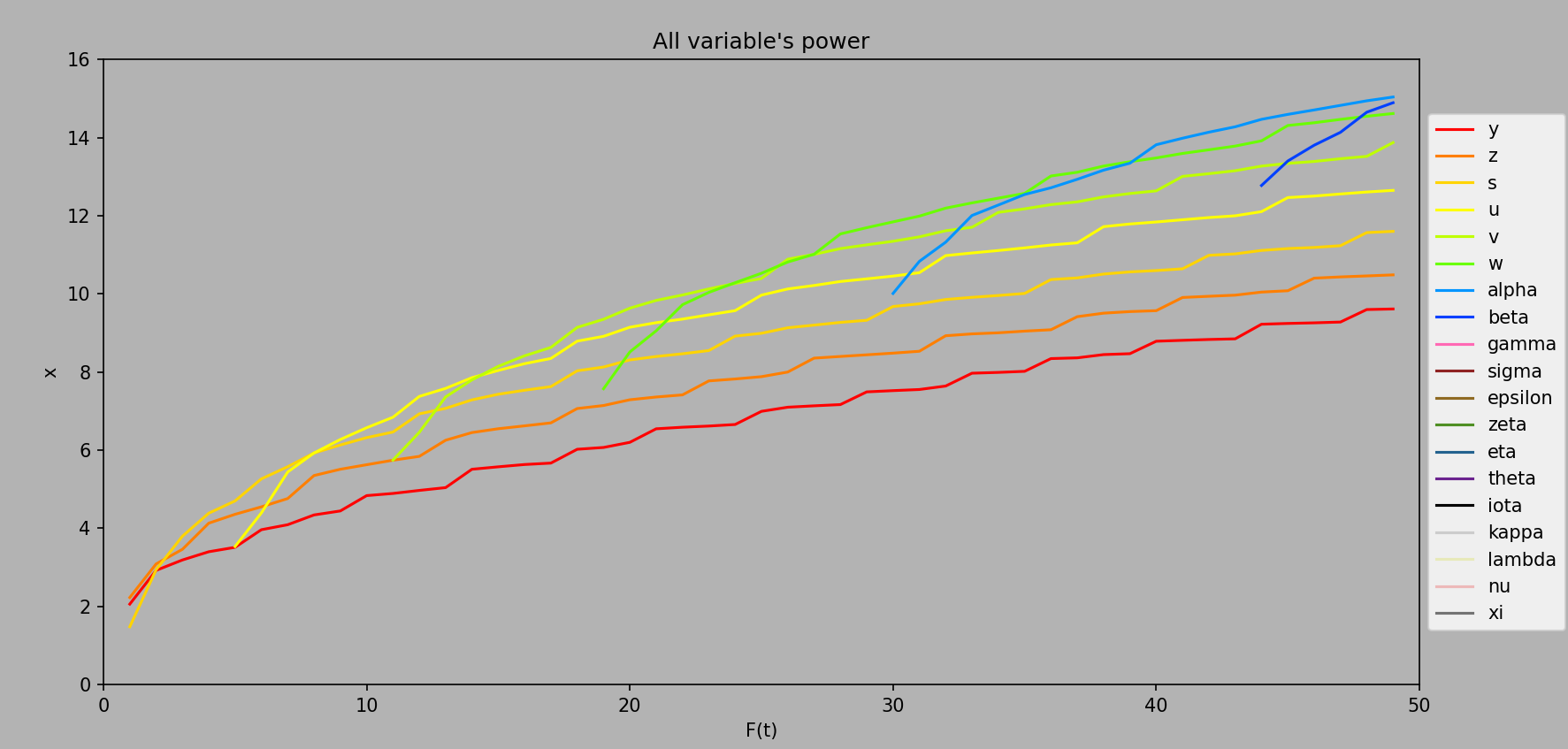
Here’s a graph of vari­able power up to ee50 $f(t)$. The ini­tial pur­chase of vari­ables $y$ through $\beta$ can be seen.

Com­puted every ee1 from ee1 to ee50.

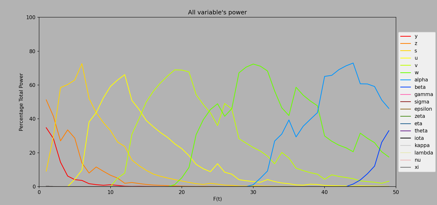
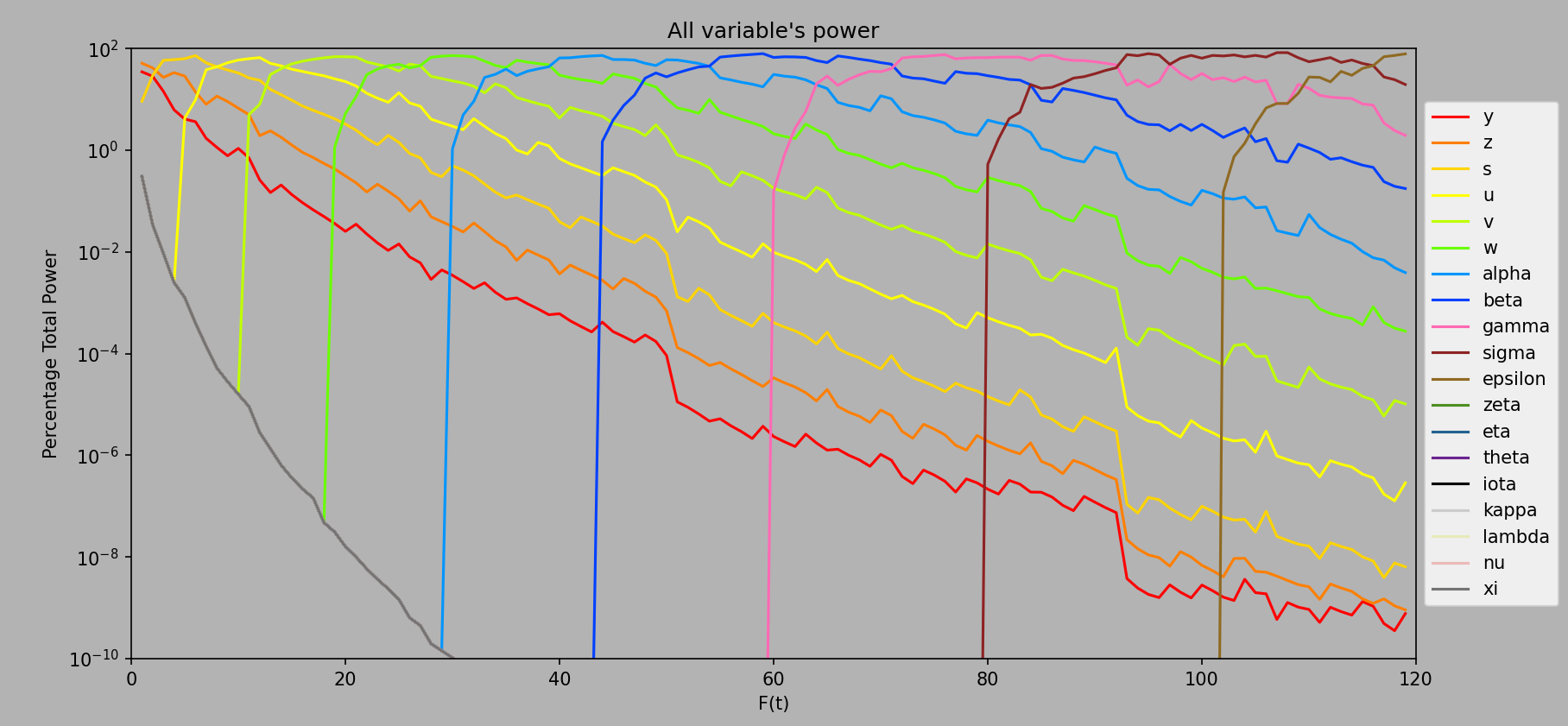
And here’s a graph with the same $f(t)$ range, but in­stead of the power of each vari­able, it graphs the per­cent­age of total power each vari­able has at any given $f(t)$.

Com­puted every ee1 from ee1 to ee50.

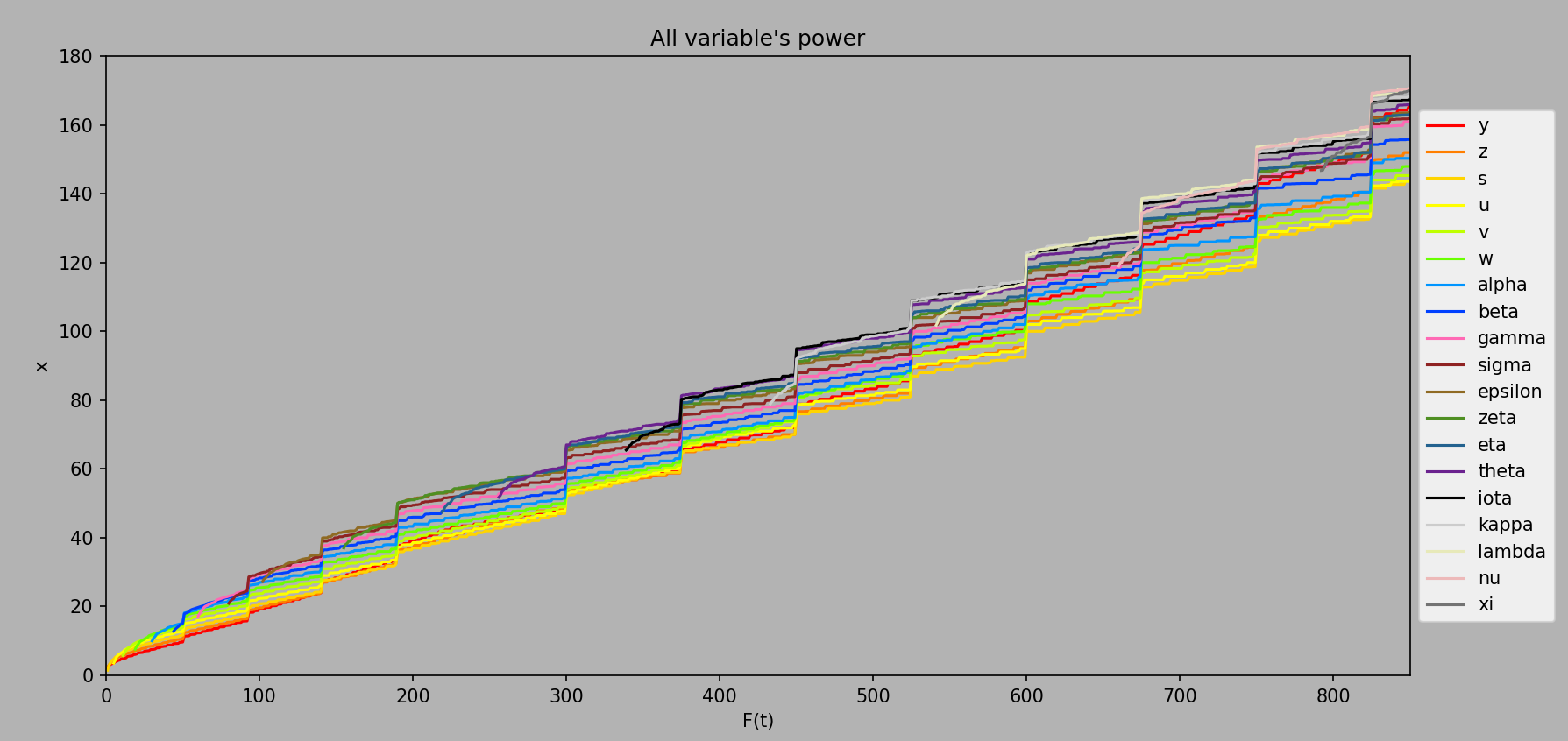
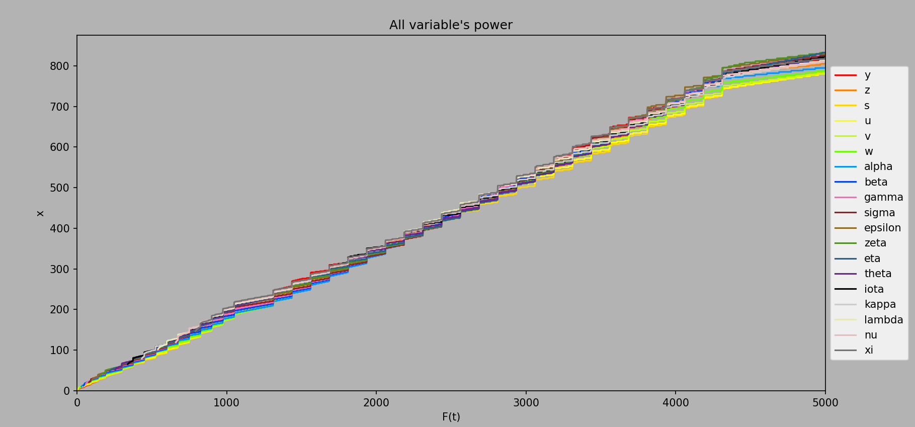
And here’s a graph of vari­able power up to the pur­chase of the fi­nal vari­able at ee791:

Com­puted every ee1 from ee1 to ee850.

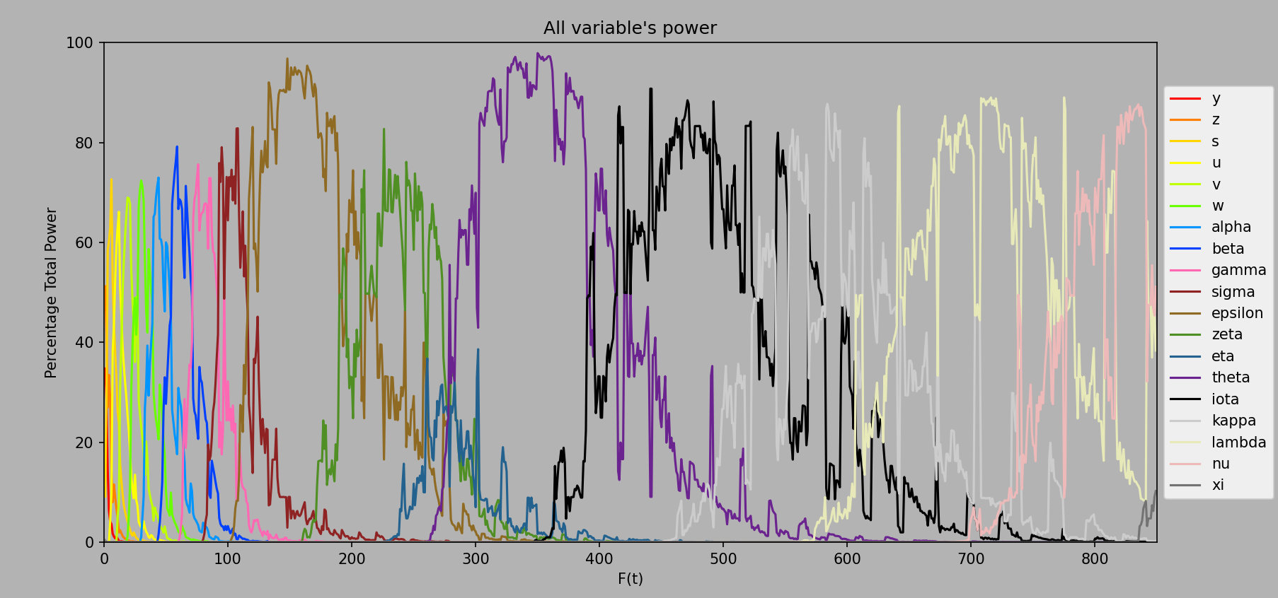
And the per­cent­age graph:

Com­puted every ee1 from ee1 to ee850. A bit more spiky ;)

$y$ Power Up­grades (ee50 - ee4310) #

You may have no­ticed the ab­rupt jumps in the above graphs. We’ll now dis­cuss why that oc­curs.

After we su­prem­acy for the first time at ee50, we are given a cur­rency $\psi$ (psi). With this new cur­rency, we can buy up­grades to in­crease the ex­po­nent on $y$. Each up­grade raises the ex­po­nent by $0.2$, so the ini­tial su­prem­acy at ee50 turns $y$ into $y^{1.2}$. These up­grades con­tinue all the way up to $y^{9.0}$ at ~ee4310, for a total of $40$ levels.

Be­cause the power each vari­able has is propag­ated down all of its lower vari­ables (ex. $z$ → $y$ → $x$), the change in ex­po­nent af­fects how strong all of the vari­ables are.

The cost of each up­grade from $y^{1.2}$ through $y^{1.8}$ is cal­cu­lated us­ing this for­mula, where x is the level you are buy­ing start­ing at 1:

$\psi =1.5\times 2^{2(x-1)}$

The cost model changes after this, and from $y^{2.0}$ through $y^{4.0}$ is this for­mula:

$\psi =0.488281\times 2^{3(x-1)}$

The cost model changes one fi­nal time, and from $y^{4.2}$ to $y^{9.0}$ is this for­mula:

$\psi =0.0000000794093\times 2^{5(x-1)}$

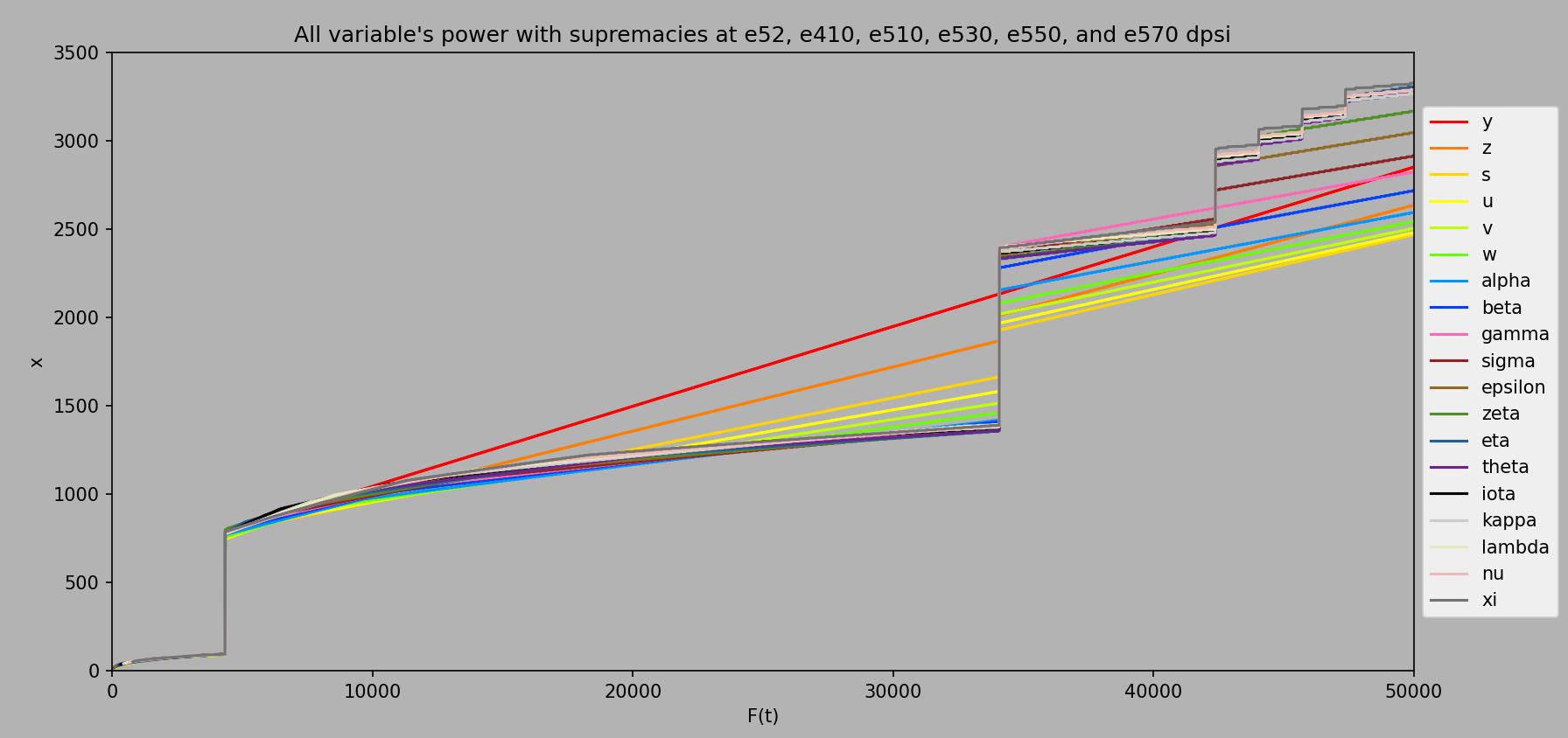
With all of these cal­cu­la­tions in place, here is the new vari­able power graph, now ran­ging up to ee5000:

Com­puted every ee1 from ee1 to ee5000.

Each small jump present in the graph marks the pur­chase of an ad­ded $0.2$ to the ex­po­nent of $y$.

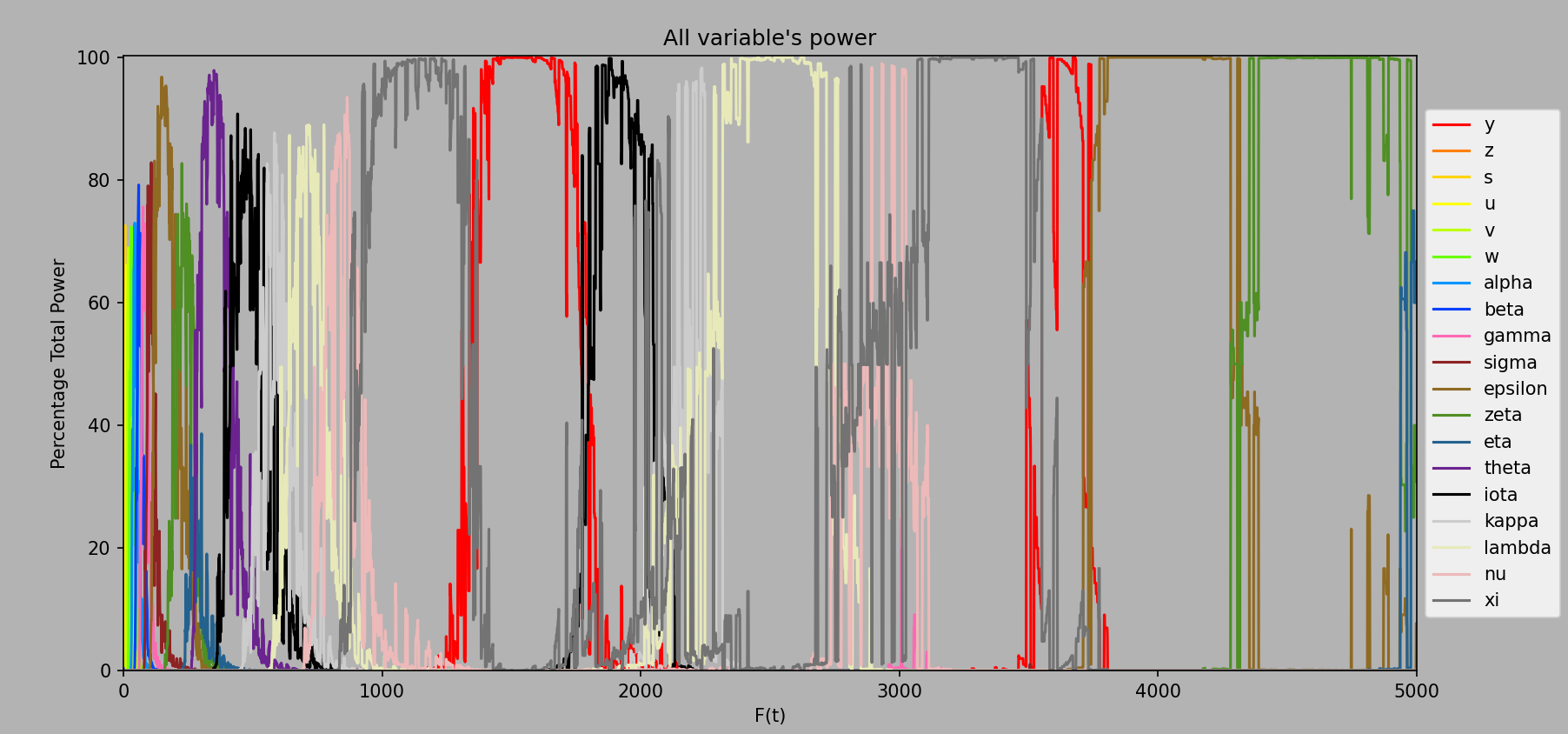
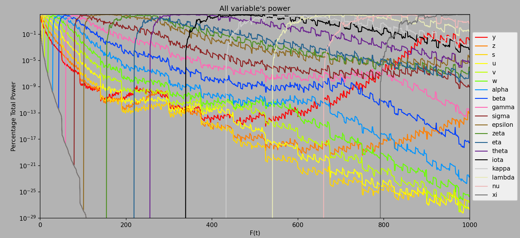
And fi­nally, here is the per­cent­age of total power for each vari­able:

Com­puted every ee1 from ee1 to ee5000.

Very spiky!

Psi3 Up­grades (ee9160 - ee47362) #

After we buy $y^{9.0}$ at around ee4310, we don’t have any­thing to buy with $\psi$ un­til ee9160 $f(t)$, when we can fi­nally af­ford the first Psi3 up­grade. This time, in­stead of 40 levels to buy, there’s only 24 up­grades. However, each up­grade is sep­ar­ated by e20$\psi$, so the last level, bought with e570$\psi$, is all the way up at ee47362 $f(t)$.

These up­grades help delay the de­cay play­ers would oth­er­wise ex­per­i­ence from ee20k-ee50k as their the­or­ies slow down and they gain less $\tau$.

The first psi3 up­grade in­creases $z$’s ex­po­nent to $z^{1.04}$, and the second up­grade in­creases it fur­ther to $z^{1.08}$. The third and fourth up­grades in­crease $s$’s ex­po­nent to $1.08$, and so on un­til the fi­nal up­grade in­creases $\eta$’s ex­po­nent to $1.08$.

To il­lus­trate the ef­fect these pur­chases have, let’s use an ex­ample.

Let’s say these are the cur­rent equa­tions for your first five vari­ables:

$x=4.7893e7y^9+2^3\times 165.2$
$y=19891z^{1.08}+2^{419}\times 87522$
$z=18082s^{1.04}+2^{376}\times 70017$
$s=16433u+2^{341}\times 56007$
$u=14933v+2^{323}\times 48973$

And let’s say that shortly af­ter­ward you pur­chased a new psi3 level:

$x=4.7893e7y^9+2^3\times 165.2$
$y=19891z^{1.08}+2^{419}\times 87522$
$z=18082s^{1.08}+2^{376}\times 70017$
$s=16433u+2^{341}\times 56007$
$u=14933v+2^{323}\times 48973$

With this new level, the power of $s$ and $u$ will in­crease, be­cause in their propaga­tion down to $x$ they get boos­ted by the ad­ded $0.04$ on $s$’s ex­po­nent. However, the power of $x$, $y$, and $z$ will get no boost, be­cause they are down­stream of the ad­ded ex­po­nent.

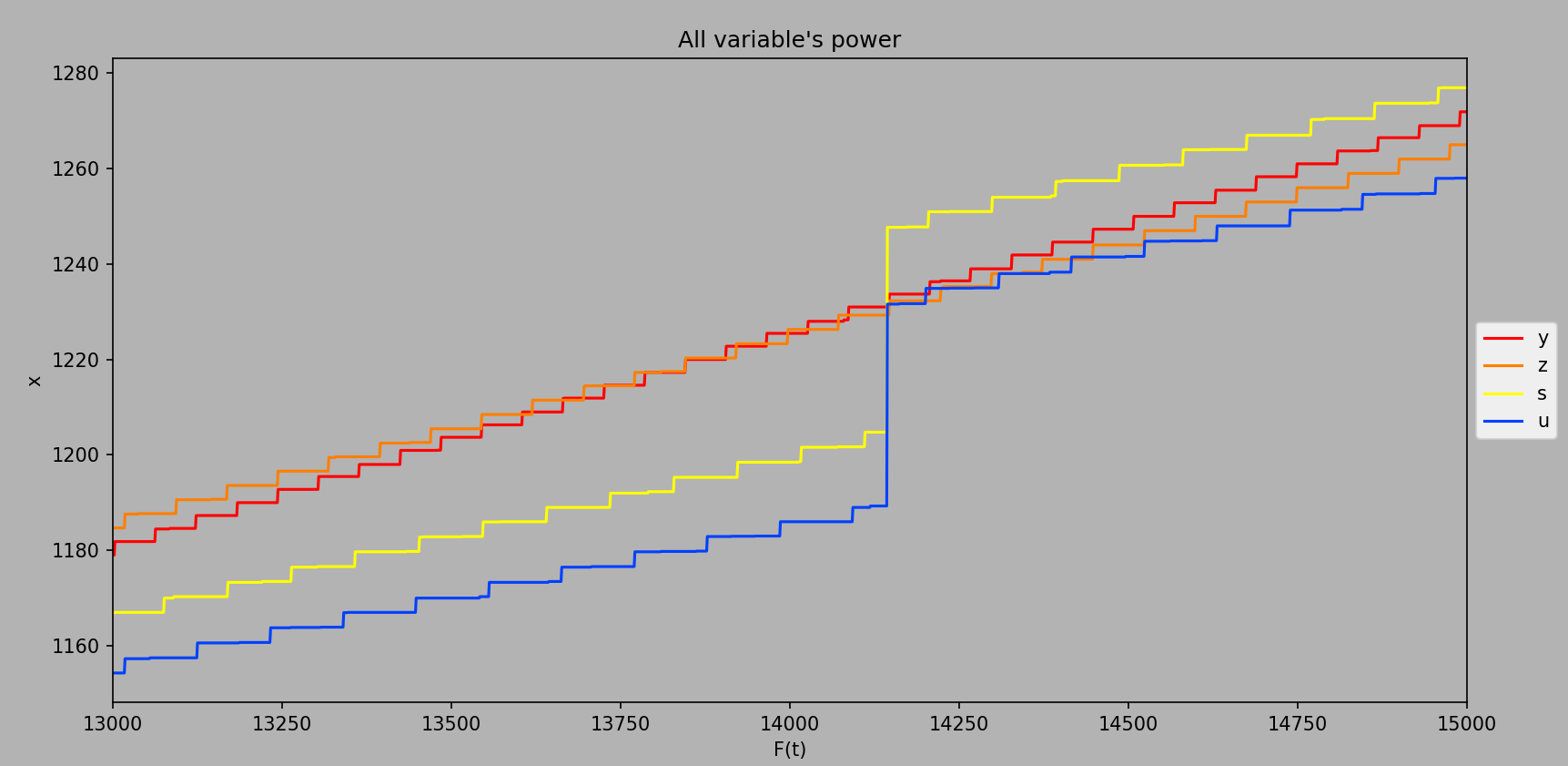
But don’t just take my word for it. Let’s look at the data from the pro­gram around this up­grade.

Com­puted every ee1 from ee13000 to ee15000. For the pur­pose of this visu­al­iz­a­tion, only the four vari­ables dis­cussed are plot­ted.

As can be seen in the im­age, both $y$ and $z$ get no boost, as we ex­pec­ted. Fur­ther­more, both $s$ and $u$ get an equal boost from the up­grade, as will the sub­sequent vari­ables all the way down to $\xi$.

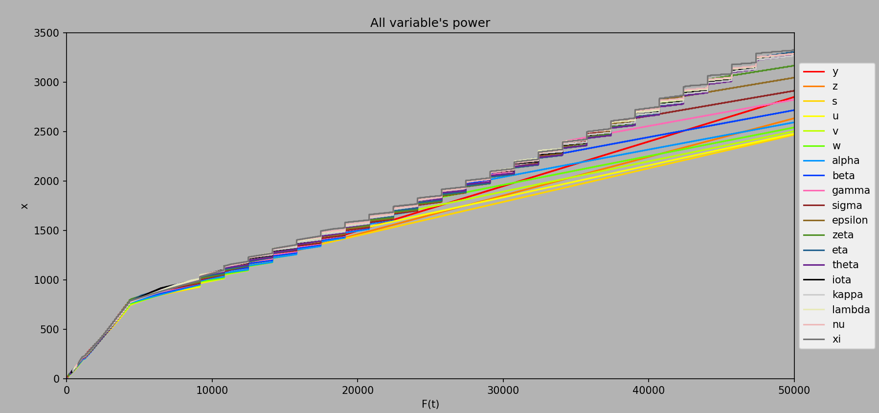
This leads to an in­ter­est­ing ef­fect where every two psi3 up­grades one of the vari­able’s power stops get­ting boos­ted from the up­grade, so we see a line sep­ar­ate from the rest every two jumps:

Com­puted every ee1 from ee1 to ee50000. This took a while to run…

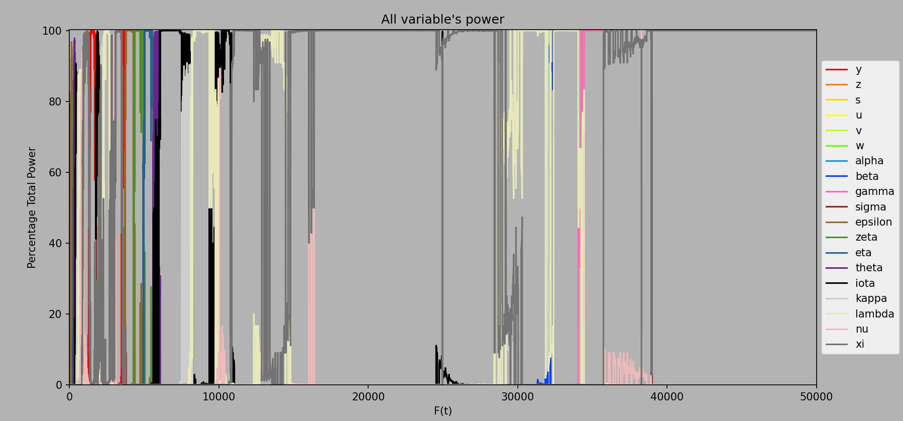
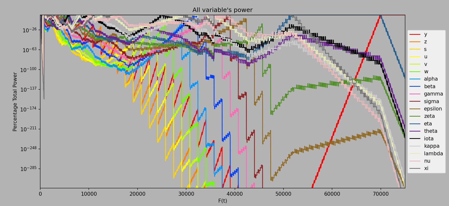
And here’s a rather in­ter­est­ing plot with the per­cent­age of total power each vari­able has.

Com­puted every ee1 from ee1 to ee50000.

Post-Psi3 Vari­able Power (ee47362+) #

We’ve made it. The end of the su­prem­acy up­grades is upon us. What’s next?

Well, now is when $f(t)$ de­cay really hits. Let’s take a look at an up­dated graph.

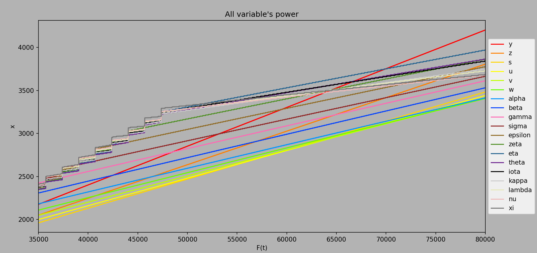
Com­puted every ee5 from ee35000 to ee80000.

Im­me­di­ately after the fi­nal su­prem­acy up­grade, we gain a lot less $x$ per $f(t)$. Dur­ing the psi3 up­grades, we need an av­er­age of $17f(t)$ for an $e1$ in­crease in $x$.

Shortly af­ter­ward, dur­ing the period up to ~ee52000, $\xi$ is the most power­ful vari­able. Un­for­tu­nately for us, its scal­ing is ab­so­lutely ter­rible, and it takes $77f(t)$ for an $e1$ in­crease in $x$, around 4.5 times worse than dur­ing the psi3 up­grades.

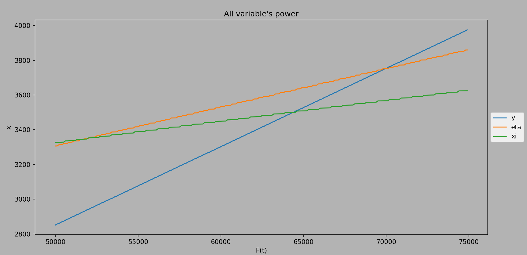
For­tu­nately, $\xi$ is quickly de­throned by $\eta$, which is the most power­ful vari­able from ee52000 all the way un­til ee70000 $f(t)$. For $\eta$, it takes $45f(t)$ for an $e1$ in­crease in $x$. This is the sec­tion where all cur­rent en­dgame and top play­ers are.

Fi­nally, at ee70000, $\eta$ is de­throned by $y$, which will re­main the strongest vari­able for the rest of the game. $y$ dom­in­ates the en­dgame be­cause for $y$ it only takes $22f(t)$ for an $e1$ in­crease in $x$, which is in­triguingly close to the $17f(t)$ the psi3 up­grades offered long ago in our dis­tant past. Cur­rently, all top lead­er­board play­ers are in this range thanks to a sig­ni­fic­ant buff to Cus­tom The­or­ies.

Class: strat; Cap­tion: $F(t)$ Needed to Gain e1 x;

A plot with only $y$, $\eta$, and $\xi$ to il­lus­trate the dif­fer­ence in their scal­ing and where each vari­able be­comes dom­in­ant.

Why We Buy $y$ Dur­ing En­dgame Gradu­ation Re­cov­ery #

Even be­fore $y$ be­comes the most power­ful vari­able, as long as you are past ee48000, you should still buy $y$ dur­ing gradu­ation re­cov­ery. Why? Well, it has to do with the su­prem­acy equa­tions we be­gin ad­opt­ing at ee48000.

At ee48000, the su­prem­acy equa­tion we re­com­mend us­ing skips most of the psi3 su­prem­acy up­grades. In fact, it only su­prem­a­cies at $e52,e411,e511,e531,e551,$ and $e571d\psi$. It does­n’t buy any of the psi3 up­grades un­til e410$d\psi$. Let’s take a look at what that does to the power of the vari­ables:

Com­puted every ee10 from ee1 to ee50000

Very in­ter­est­ing! So it looks like we should be buy­ing $y$ un­til the su­prem­acy at e410$\psi$. When we were buy­ing every psi3 up­grade, it was­n’t worth buy­ing $y$ be­cause the other vari­ables were stronger than it. However, these vari­ables were only stronger than $y$ be­cause they had been boos­ted by the psi3 up­grades, none of which af­fect $y$’s power.

After we reach ee52000, we are re­com­men­ded to use a new su­prem­acy equa­tion. This equa­tion only su­prem­a­cies at e52, e511, and e571 $d\psi$. Let’s see what that does to the power:

Com­puted every ee10 from ee1 to ee50000

Once again, it looks like we should be buy­ing $y$ dur­ing gradu­ation re­cov­ery. This time, we should be buy­ing $y$ un­til the e510$\psi$ su­prem­acy.

Fi­nally, some­where between ee58000 and ee60000 (we aren’t en­tirely sure where within this range) we switch to our fi­nal su­prem­acy equa­tion. This su­prem­acy equa­tion only su­prem­a­cies at e52 $d\psi$ and e571 $d\psi$.

Com­puted every ee10 from ee1 to ee50000

There we go! Now we should buy $y$ all the way up to e570$\psi$.

Ad­di­tional Graphs #

Where I put all of the in­ter­est­ing plots that did­n’t fit well in any sec­tion.

Full Graph
The plots of vari­able power from ee1 to ee75000.

Com­puted every ee5 from ee1 to ee75000.

And the plot with per­cent­age of total power for each vari­able:

Com­puted every ee5 from ee1 to ee75000.

Log Per­cent­age Total Power Plots #

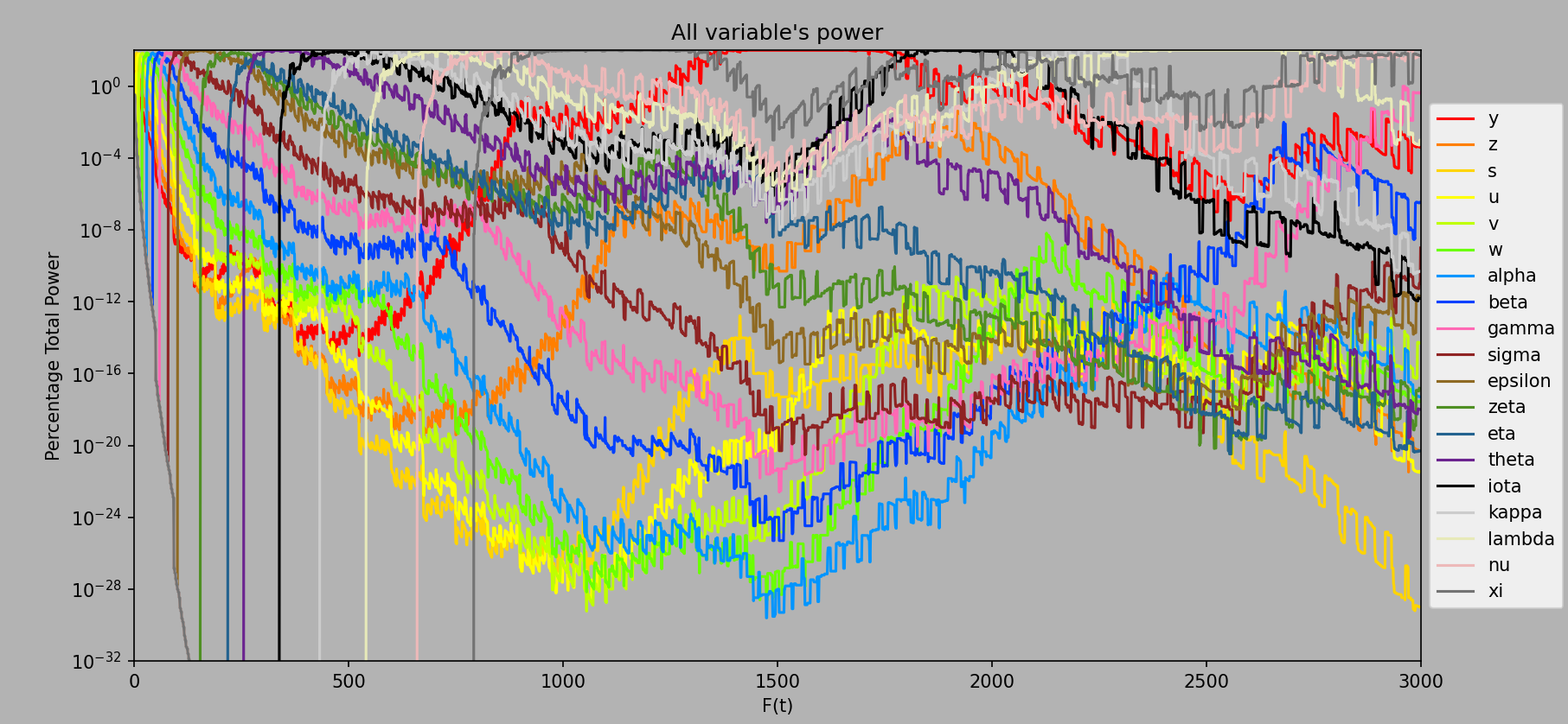
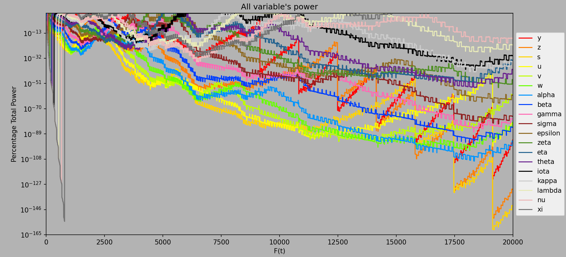
More than just the reg­u­lar per­cent­age total power plots, I also tried log­ging the per­cent­age so we can see more than just 0% power for al­most all of the vari­ables, cre­at­ing fas­cin­at­ing res­ults. Ig­nore the ini­tial xi/ $\xi$ line in the first im­age; it’s a rem­nant that only shows up in these logged plots.

Com­puted every ee1 from ee1 to ee120.

Com­puted every ee1 from ee1 to ee1000.

Com­puted every ee1 from ee1 to ee3000.

Com­puted every ee1 from ee1 to ee20000.

Com­puted every ee10 from ee1 to ee75000.

So many stor­ies told in one plot!