Ex­po­nen­tial Idle Ba­sics

Guide writ­ten by LE★Baldy and Snaeky. Con­tri­bu­tions from The Amaz­ing Com­munity.

This guide is cur­rently un­der­go­ing change. Keep in mind, strategies may change.

Feel free to use the gloss­ary as needed.

This in­tro and fol­low­ing guide are de­signed to help you play through the 1 to ee2000 sec­tion of the game. This in­tro­duc­tion will give you some fun­da­ment­als to help you pro­gress while play­ing this sec­tion of the game.

If you don’t want to have spoil­ers for the later game, don’t read fur­ther ahead than you are already.

Vari­ables and Up­grades #

• Vari­ables are the main pur­chases in the game. They will be the most im­port­ant to buy, and you should buy them as pri­or­ity be­cause they in­crease Life­time f(t) faster. All of the vari­ables pur­chas­able are be­low. You will not be able to get all of them right away but will be able to get them all as you keep play­ing. This screen is found by press­ing the <Up­grades> but­ton between the up­grades and the main equa­tion graph.
• Up­grades are where ad­di­tional boosts to vari­ables lie. They are cru­cial to pro­gress and should be bought of­ten. You will be able to see items that can be pur­chased with f(t), \(\mu\), and \(\psi\) on that page in that or­der. You can nav­ig­ate to that tab by press­ing the <Vari­ables> but­ton between the vari­ables and the main equa­tion graph.

Vari­able Names #

What does ee mean? #

You start out with nor­mal num­bers and quickly work your way up to \(X.xxeX\) nota­tion. This nota­tion is sci­entific nota­tion. It stands for \(X.xx*10^X\). Later you are in­tro­duced to \(X.xxeeX\). This is a cus­tom game nota­tion that stands for \(X.xx*10^{10^X}\).

Achieve­ments and Minigames #

• Achieve­ments are just that. They are goals to reach that give you stars as re­ward.
• Minigames are puzzles that you can solve that will give you stars as a re­ward for get­ting solv­ing them. Check out the Minigame Guide for how to solve each puzzle and more re­sources.

Stars and Star up­grades #

• Stars are a cur­rency that op­er­ates out­side of the main game that you use to pur­chase star up­grades. These up­grades range from QoL (Qual­ity of Life) fea­tures to boosts to the game­play. For the most part, you should pri­or­it­ize new vari­ables as soon as you can, EX­CEPT for Auto­prestige. Auto­prestige is a huge boost in pro­gress due to im­possible to rep­lic­ate levels of op­tim­iz­a­tion, and you should pri­or­it­ize it over vari­ables of a sim­ilar cost. More de­tails on star up­grades to pri­or­it­ize can be found in fol­low­ing guides.

Auto­prestige ex­pres­sion #

timer(pt * d(ln(ln(db / b + 1))) < 1)
> 3 * tr && db > b

Copy Text

Auto­prestige ex­plan­a­tion #

The idea be­hind \(d(ln(db/​b+1)/​pt) < 0\) is clearer if you con­sider a dif­fer­ent term \(d((db/​b+1)^{(1/​pt)}) < 0\). They meas­ure the same thing, but the second one is just raised to the ex­po­nent, base e. They are equi­val­ent be­cause \(e^x\) (and \(ln (x)\)) are both strictly in­creas­ing func­tions on the do­main \(x > 0\), so ap­ply­ing those func­tions will not change where the local max­imum is loc­ated (when \(d\) changes sign).

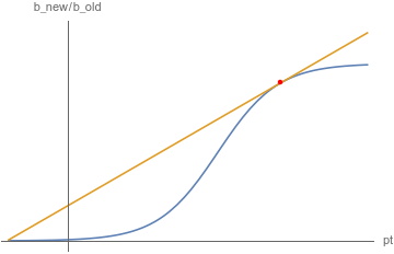
\(db/​b+1\) is bet­ter ex­plained with \((b + db)/​b\). \(b + db\) is the new \(b\) value you would get after prestige, and \(b\) is the old \(b\) value you cur­rently have. If you prestige, your \(b\) is mul­ti­plied by that ex­act value. That is, your \(b\) grows with ra­tio \((b + db)/​b\) if you were to prestige.

The gen­eral idea of a good ex­pres­sion would be to “max­im­ize \(f\) growth over time,” and it would be the same as “max­im­ize \(b\) growth over time.” To meas­ure \(b\) growth over time, in this ap­proach we take the growth of \(b\) that can res­ult from cur­rent prestige only and take \((b + db)/​b\) as the ra­tio of growth.

We could di­vide the ra­tio by time, but that does­n’t make sense be­cause ra­tios are ap­plied mul­ti­plic­at­ively (e.g. ra­tio \(r\) per second means \(r^5\) in \(5\) seconds, not \(5*r\)). Hence, in­stead of di­vid­ing, we take the power \(1/​pt\) (\(pt\) be­ing the time since prestige) to get the cor­rect value of ra­tio.

There­fore, we get the ex­pres­sion \(((b + db)/​b)^{(1/​pt)}\) which rep­res­ents “after last prestige, \(b\) grew by \(this\) \(ra­tio\) per second.” To max­im­ize this value, we note that this value ac­tu­ally achieves one local max­imum (by work­ing through the be­ha­vi­ors of (\(f\) over time) so we may simply take a de­riv­at­ive (\(d\)) and see when it turns neg­at­ive.

Visual rep­res­ent­a­tion #

Auto­su­prem­acy ex­pres­sion #

timer(pt * d(ln(ln(db / b + 1))) < 1)
> 3 * tr && db > b
&& dpsi + psi > min(min(cos­tUpS(1),
cos­tUpS(2)), cos­tUpS(3))
&& ln(1 + max(1, lo­g10(sf)) /
smooth(max(1, lo­g10(gf)),
(st > tr) * ee99)) / max(1, st) <
smooth(ln(1 + max(1, lo­g10(sf)) /
smooth(max(1, lo­g10(gf)), (st > tr)
* ee99)) / max(1, st), (pt > tr) * ee99)

Copy Text

YOU NEED TO MANU­ALLY SU­PREM­ACY WHEN YOU PUT THIS INTO YOUR GAME!

Ref­er­ence Lock­ing Smooth()

Auto­su­prem­acy ex­plan­a­tion #

The auto­su­prem­acy ex­pres­sion is an at­tempt to do the auto­prestige ex­pres­sion, but for su­prem­acy. It tracks the same in­form­a­tion, but over mul­tiple prestiges. It is harder to make an auto­su­prem­acy ex­pres­sion than an auto­prestige ex­pres­sion be­cause after a new prestige, Su­prem­acy \(f(t)\) does­n’t in­crease un­til you get back to the \(f(t)\) you left off at. This cre­ates the growth of a su­prem­acy stair­case shaped. This makes it dif­fi­cult to find the op­timal point as we did with auto­prestige and is why we time it with the end of a prestige to be sure.

Smooth() for auto ex­pres­sions #

In­tern­ally, smooth is im­ple­men­ted us­ing ex­po­nen­tial mov­ing av­er­age. Here are some ways to use this con­struc­tion.

Method 1: Mov­ing av­er­age #

If a value fluc­tu­ates too much, you can use smooth so that the value does not go rampant, trig­ger­ing some con­di­tions in­cor­rectly. One main ex­ample is to use it when you use mul­tiple \(d()\) func­tion on the same ex­pres­sion.

For in­stance, \(smooth( d(d(ln(db))), 10)\) will be­have much bet­ter than the simple \(d(d(ln(db)))\) be­cause us­ing d mul­tiple times cre­ates a lot of fluc­tu­ation, due to the dis­crete nature of \(d()\) (not a true de­riv­at­ive, but an ex­tra­pol­a­tion of slope over the last tick). Of course, this in­tro­duces some “lag factor” in the sense that when some threshold is passed, smooth won’t dis­play it un­til a short after.

Method 2: Lock #

Due to the nature of the ex­pres­sion, if the second in­put of smooth is very large, then there will be no av­er­age at all: in­stead of tak­ing a nor­mal av­er­age, we can skew the weights so that any new value is too small to be no­ticed. As a very simple ex­ample, we can cal­cu­late av­er­ages like \(av­er­age = 0*(new\) \( value)+1* (old\) \( value)\) to pre­serve old val­ues. On the con­trary, if we skew this the other way, then only the new value would ap­pear: \(av­er­age = 1*(new\) \(value)+0* (old\) \( value)\).

A simple ex­pres­sion like \(smooth(expr, ee99)\) will first com­pute expr and keep that value in­def­in­itely un­til the ex­pres­sion field is re­set: upon modi­fy­ing the ex­pres­sion, every prestige for prestige ex­pres­sions, and every su­prem­acy for su­prem­acy ex­pres­sions. This is what we refer to as “lock.”

However, we can do bet­ter: in­stead of simply lock­ing val­ues, we can con­trol when the lock­ing mech­an­ism comes in. Us­ing con­di­tions, we can switch back and forth between in­def­in­ite locks and in­stant­an­eous up­dates: \(smooth(expr, ee99*cond)\). If cond is true, then \(ee99 *cond\) will be ee99, thereby ac­tiv­at­ing the lock. If cond is false, then \(ee99 * cond\) will be 0, thereby switch­ing to in­stant­an­eous up­dates. The res­ult is that we ob­tain the value of expr eval­u­ated when the cond was last false.

Method 3: Cu­mu­lat­ive max­imum #

If we have two really large val­ues, the av­er­age of the two will be in fa­vor of the lar­ger of the two. In fact, if the two num­bers are really really big, the av­er­age will be in­dis­tin­guish­able from the lar­ger of the two due to fi­nite data stor­age (term: float­ing point pre­ci­sion). We can ab­use this idea to con­vert the in­put of smooth into a very large value, thereby con­vert­ing av­er­ages like \(av­er­age = 0.5 *(new\) \(value) + 0.5 * (old\) \( value)\) into the equi­val­ent \(av­er­age = max(new \) \(value, old \) \(value)\). The ef­fect is that we ob­tain the max­imum value that the in­put at­tained ever since the ex­pres­sion was re­set (from modi­fy­ing the ex­pres­sion or from prestige (resp. su­prem­acy) for prestige ex­pres­sion (resp. su­prem­acy ex­pres­sion)). Of course, we have to can­cel out the mag­ni­fic­a­tion of the in­puts in or­der to re­trieve the value we ac­tu­ally want.

For ex­ample, \(smooth(10^{10^{10^{db}}}, 1)\) has the in­put large enough that it dis­plays the largest value of \(10^{10^{10^{db}}}\) that oc­curred so far. However, we would­n’t want db blown up this way, so we can use \(log_{10}(log_{10}(log_{10}(smooth(10^{10^{10^{db}}}, 1))))\) to re­trieve back the max­imum \(db\).

Ref­er­ence for­mula #