Custom theories are theories made by players in the community. As of March 2025, there are 9 official custom theories that contribute up to e600 per theory; Weierstrass Sine Product made by Xelaroc (WSP), Sequential Limits by Ellipsis (SL), Euler’s Formula by Peanut, Snaeky, and XLII (EF), Convergents to Square Root 2 (CSR2/CS2) by Solarion, Fractional Integration (FI) by Gen and Snaeky, Fractal Patterns (FP) by XLII, Riemann Zeta Function by Prop (RZ), Magnetic Fields by Mathis (MF) and Basel Problem by Python’s Koala (BaP). The theories will be abbreviated as WSP, SL, EF, CSR2, FI, FP, RZ, MF and BaP from now on. The choice for a three letter abbreviation for BaP was made to avoid confusion with a previous unofficial custom theory sharing the same initials (Bin Packing).
In order to balance custom theories with the main theories in the endgame, custom theories have a low conversion rate (with two exceptions) from to . WSP, SL, CSR2, FI, RZ and BaP have conversion rates of = while EF has a conversion rate of = and FP with a conversion rate of = . Meanwhile, MF is the only custom theory to this day to have = .
In general, you want to be as efficient as possible since R9 does not affect custom theories. If you cannot be active, try not to do an active theory or do an active strategy. Some custom theories are more active than normal theories and it is highly suggested that if you are doing active strategy for a Custom theory (SL or FI before all milestones, MF, CSR2, WSP, or early FP) that you do an idle main theory (such as T2, T4, or T6) so that you don’t miss out on .
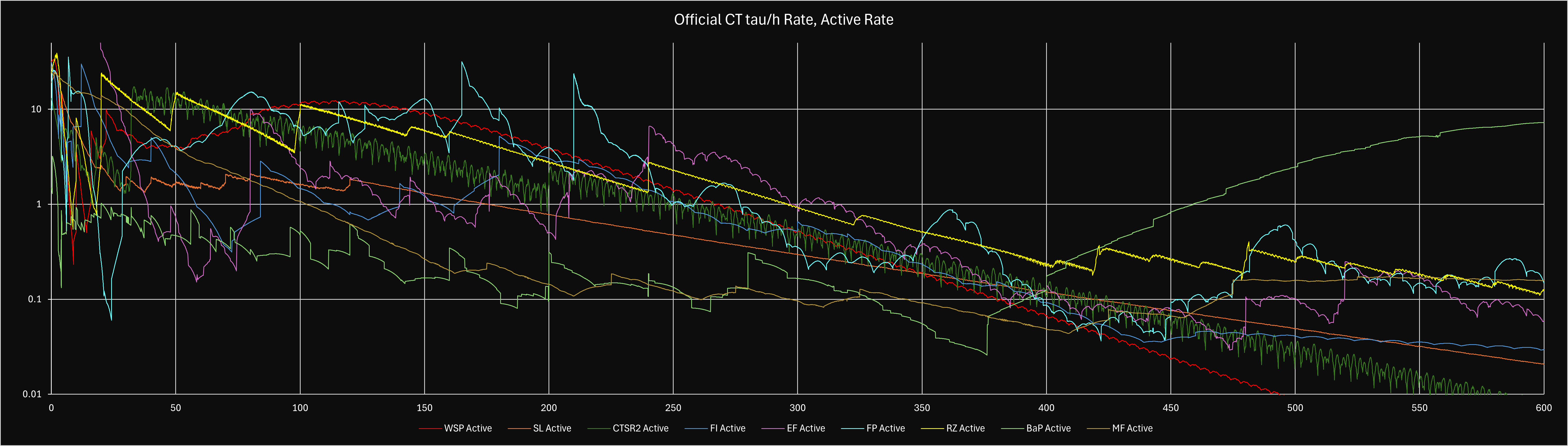
If you have time for active strategies, try to do the CT with the highest active , or you can chase a spike in , such as EF e50 or FP e95 . You can check this with the sim.
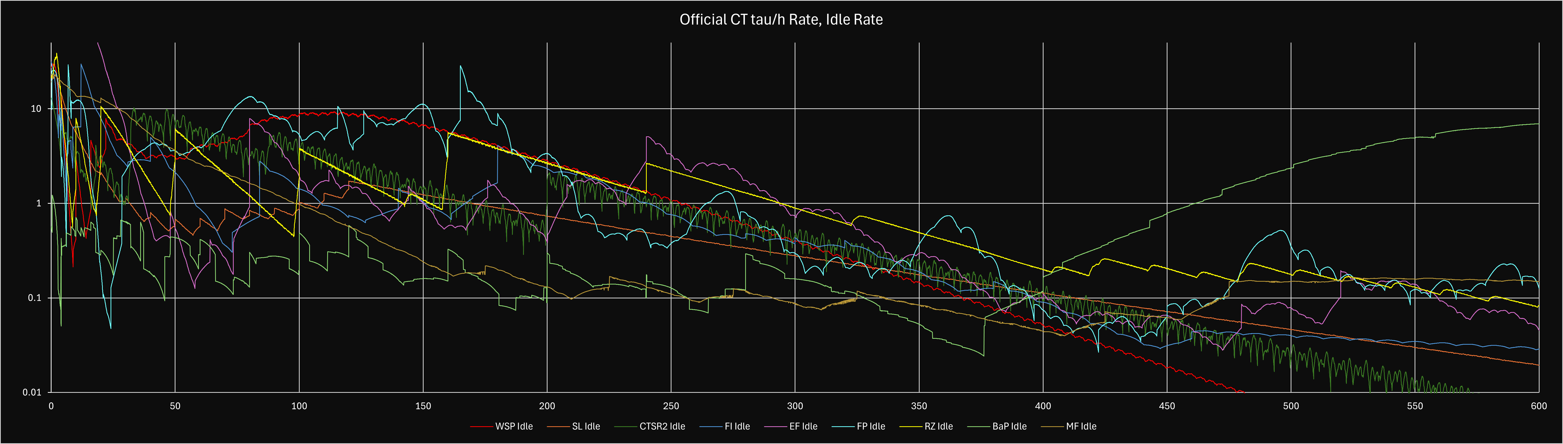
For idle time, do the one with the highest idle , (or the longest publication time if you’re doing overnights), with preference toward EF, SL, BaP, FP past e1050, or FI when you only have 1 milestone to swap. For example, if SL has 2 and CSR2 also has 2 , ideally we would pick SL. The reason we prefer SL, EF, FP, FI and BaP is because these theories contain multiple growing variables. This means the theories generally require less babysitting as the variables grow by themselves. The assumption of daytime idle is that we can check and publish a theory every 2 hours or so. If you can only check every 8 hours idle, please see the overnight strategy just above.
The very first official custom theory; WSP was developed by Xelaroc, who also came up with some of the strategies used in the theory. The idea behind the theory is to use the factorization of sine to increase . There are multiple equations with this theory, and some may look daunting, so we’ll have a look at each one.
The first line states that the rate of change in is . Initially it’s simply without any exponent. With milestones we add more exponents.
For the second line, the higher the (spelled ‘chi’, pronounced as ‘kai’), the higher the . We want to increase by increasing and . The signs of and will always match, so the fraction can’t be negative. Additionally, the variable is a milestone which is not initially available.
The third line is the most complicated. Generally we can factorize an equation when its graph touches the x-axis. For a sine curve, it touches the x-axis starting from x = 0, and repeats every x= . These multiplied factors form the basis of the Weierstrass Sine Product. A simpler interpretation is that we can see ‘x’ appearing both outside and inside the products in the numerator. Since is ‘x’ here, the higher the , the higher the as stated earlier.
Finally, the actual equation: increasing and increases . Note that from the fraction, we don’t want to increase only or only . Rather we should increase both. Using standard strategies this should be no problem. The part in the denominator is a milestone term. This means that is better than as more milestones are accumulated.
Approximate variable strengths on with all milestones are as follows:
Brief summary of variable strengths of WSP
Variable Description
~7% increase to on average.
Doubles (instantaneous).
Initially ~50% increase similar to . Slowly ramps up to 4x increase in . At , it is very close to a 4x increase.
Initially ~50% increase. Tends to 0% as increases. At , the increase is not noticeable anymore. Early into WSP, still buy them throughout. Late into WSP, only buy for the first ~20 seconds of each publication.
Before you get e400 for idle, simply autobuy all.
Once you have e400 , starts to become extremely bad. Because of this, the new idle strategy would be to autobuy all for 20 seconds or so. Then turn OFF. Continue to autobuy the rest of the variables.
For a simple active strategy before e400 , simply autobuy and since they double the rates long term. and give approximately 60% boost (with becoming more powerful with milestones and vice versa for ). We will buy and when their costs are less than 50% of the minimum of and .
For , we will buy it when its cost is less than 10% of the minimum of and . For example, if costs and costs , we would not buy as it’s ‘too expensive’ compared to .
For active strategy, starts to become more powerful than . If their costs are similar, we will prioritize first. For example, if costs and costs , we will buy first. Similarly to the idle strategy, we will buy only for the first 20 seconds or so. If you want more information on the different strategies pertaining to WSP, please see List of theory strategies.
SL, the second official custom theory, uses a variation of Stirling’s formula to approximate Euler’s number (). As upgrades are bought, the approximation becomes more precise, increasing and because approaches 0. As with the first official custom theory (WSP), there are several equations in this theory. Let’s explore each one:
The first line is the main part of the equation. We want to maximize to increase . The ‘1.06’ exponent is from milestones. The default is no exponent. From the equation, we can see that is proportional to approximately . This means that if we quadruple , we would approximately double long term. The denominator of the fraction has a gamma symbol () which looks like the letter ‘y’. As our increases, our becomes closer to ‘e’, so the denominator will decrease, which increases . We will explore in the next equation.
The second equation refers to Stirling’s approximation of Euler’s number ‘’. As increases, converges to Euler’s number. Long term we can approximate this convergence as linear. The implication is if we double , will be twice as close to Euler’s number, so in the first equation will be halved.
The third equation relates with and some upgrades. The most interesting part is the exponent part containing . The negative exponent actually implies that as increases, DECREASES. If is high, doesn’t grow as fast (it still grows). This has implication on the first equation as well, since depends on , which depends on .
The fourth equation relates with some upgrades. This one is relatively simple; increase and to increase . The ‘1.04’ exponents are from milestones.
The final equation simply states the value of . The lower the better. Default without milestone is .
All variables in SL are about the same in power, except for and (which are slightly worse than and . Selectively buying variables at certain times (active) yields very little results. Therefore, we can get away with autobuy all for idle. Before autobuy, simply buy the cheapest variable. If you want more details on SL strategies, in particular the execution of various strategies, please see List of theory strategies.
For active, there is a milestone swapping strategy that is significantly faster than idling (approximately twice the speed). If we carefully examine the effects of each milestone, we can conclude the following:
1st milestone: Increases exponent and increases straight away. The actual value of does not increase.
3rd/4th milestone: Increase / exponents, and , and . This also increases . However, the effect is long-term and not instantaneous unlike the effect of the 1st milestone.
We have different milestones which affect the same thing (), but one is instantaneous, while the other builds over time. This forms the basis of ‘milestone swapping’, swapping milestones at certain times to maximize per hour. If you’ve done T2 milestone swapping, this should be familiar.
We initially put our milestones in the 4th and 3rd milestones. Once our doesn’t increase quickly anymore, we switch milestones to the 1st one to gain a burst of . Once our is not increasing quickly anymore, we switch back to the 4th and 3rd milestone!
x>x>x>x represent the max buy order of milestones not the amount allocated.
For example, 4>3>1>2 means “Allocate everything into 4th milestone, then use leftovers into 3rd milestone, then into 1st milestone, then into 2nd milestone”.
At this point, the theory becomes very idle. We simply autobuy all variables. Publish at approximately 8-10 multiplier. If you wish to improve efficiency, disable & at about 4.5 publication multiplier and & at 6.0 multiplier until publish.
This custom theory, along with Convergents to Square Root 2, were released at the same time and is based on Euler’s Formula of
, where ‘i’ is the complex number.
EF is unique, along with FP, in that all the milestone paths are locked, so there’s no choice in which milestones to take. This was deliberately done to prevent milestone swapping strategies and to balance the theory. Furthermore, the to conversion for this theory is uniquely at rather than the usual meaning that less is needed to get an equivalent amount of . Due to the conversion rate, EF can feel extremely slow in comparison to other theories, but it has the largest instantaneous jump in out of all custom theories.
The first line is the main equation. We want to maximize . All the terms and their exponents are obtained from milestones. Parts of the square root term are also obtained from milestones. Note that the and the terms are effectively redundant at all stages of this theory; but due to them purchasing and respectively, they are very important.
The second line defines the graph shown. Since is graphed on the complex over time, it is possible to have it show as a particle spiraling through space.
The third line describes and , which are used to generate ‘’ and ‘’ currencies. This line by itself doesn’t do much.
The fourth line simply describes . This is used in the first equation directly.
The fifth and final line use the results from the 3rd line, so effectively and .
Approximate variable strengths on with all milestones are as follows:
Brief summary of variable strengths of EF
Variable Description
Makes increase faster. Since there are only 4 levels, after a certain point, this variable is effectively fixed.
Doubles every 10 levels. ~7% increase in per level over time.
Doubles in value every level. Also doubles per level over time.
Costs to buy. ~14% increase in per level.
Costs to buy. ~20% increase in per level.
Costs to buy. ~14% increase in per level.
Costs to buy. ~20% increase in per level.
Doubles every ~10 levels. Costs to buy. With full milestones, ~11-12% increase in .
Costs to buy. Increases 40x every 10 levels. However, note that some levels are more impactful than others, specifically . Overall, this variable ranges from 10-700% effectiveness in .
Costs to buy. With full milestones, approximately triples .
Initially, you only have , , and unlocked. Buy at about 1/8th cost of , and buy when it’s available. At e20 when autobuyers are unlocked, for idle, simply autobuy all. For active, continue to do what you were doing (buying at 1/8th cost of ). There are also more advanced strategies, in particular EFAI. For its description and execution, please see List of theory strategies.
The first 2 milestones are redundant by themselves. The term and the term are insignificant compared to the term.
Once you unlock the 3rd milestone ( term) however, we can buy at 1/4th of cost.
This custom theory was released at the same time as Euler’s Formula. CSR2 is based on approximations of using recurrent formulae. As the approximations improve, the and improve, increasing . An explanation of each section of the equations is shown below:
The first line is self explanatory. The exponents on are from milestones. ‘’ will increase during the publication.
For the second line, both the variable and its exponents are from milestones. The absolute value section on the right describes the approximation of / to . As / get closer to , the entire right section gets larger and larger (because of the -1 power).
The third and fourth lines are recurrence relations on and . This means that the current value of and depend on their previous values. We start with = 1, = 3. The equation will then read as:
.
Then .
Similar logic is applied to equations.
This occurs until we reach and reach whatever ‘m’ values we have. This is shown in the next equation:
The fourth equation relates ‘m’ as described above. We can see that as we buy and , our will increase, so the 2 recurrence equations above will ‘repeat’ more often and , will increase. From how and values are calculated, buying 1 level of or will increase by 1.
For idle, autobuy all. The idle strategy doesn’t change much. If you would like to be more efficient while still being idle, remove milestones and stack them into the exponent milestones when you are about to publish (from around e80 to e500). Don’t forget to change milestones back after publishing!
The active strategies are significantly more involved. Depending on how active you would like to be, there are several potential strategies. There’s the standard doubling chasing CSRd, which is just autobuy all except and , where you buy them when they are less than 10% cost of minimum(, , and ).
For the milestone swapping strategy, the general idea is to switch milestones from and its exponents, to exponent milestones whenever we are ‘close’ to a powerful upgrade. Please see the Theory Strategies section of the guide for how to perform milestone swapping.
This theory has a milestone swapping strategy before full milestones. We have exponent milestones, which increase straight away. We also have related milestones, which increases the variable, which increases .
The reason milestone swapping works is because the benefits of using related milestones (having high ) remain when you switch to exponent milestones. If we only use exponent, then we have really low . If we only use related milestones, then we have high , but low . If we regularly swap them, we can increase through related milestones, then take advantage of the exponent milestones, while keeping the high value of we’ve accumulated earlier!
For a more detailed explanation on how to actually do the strategy, please see the Theory Strategies section of the guide.
This custom theory was released at the same time as Fractal Patterns. FI is based on Riemann–Liouville Integrals and allows you to approach the full integral as the fraction approaches 1. An explanation of each section of the equations is shown below:
Note: The bounds of the integral change from after 3rd milestone.
Equations
Milestone 0
Milestone 1
Milestone 2
Milestone 3
Equations
Milestone 0
Milestone 1
Milestone 2
The first equation is for , which starts off simple, but gets more complicated as more milestones are reached and perma-upgrades are purchased. Initially, is fairly simple to calculate as is just , is just the variable, and the radical is just / where is just . However, once is added to the equation, the radical becomes which can be estimated by raising to the highest power of by 1 and upon maxing out the milestone, it becomes . The variables and are simple multipliers that do not change over time without purchasing them with .
The second equation is for , which seems simple at first, but gets more difficult to understand once we get to the fractional integral. The notation in game is rarely used, but it is used to save space. Tapping and holding the equation will give the full equation. When increases, the fractional integral approaches 1, which makes the fractional integral get closer to, yet still smaller than, the full integral. By subtracting the two, then dividing 1 by the difference, we get a very large number.
For idle, autobuy all. The idle strategy doesn’t change much other than not doing Milestone Swap. If you are able to check in every 30 minutes or so, manually buy and . Make sure that to autobuy when close to getting a boost.
The active strategies are a bit more involved. Depending on how active you would like to be, there are several potential strategies. There’s the standard doubling chasing FId, which is just autobuy all except and , where you buy them when they are less than 10% cost of minimum(, , and ).
For the milestone swapping strategy, the general idea is to switch milestones from , to / milestones whenever we gain 3x to after purchasing , or some gain adjusted for from purchasing . Please see the Theory Strategies section of the guide for how to perform milestone swapping.
This theory has a milestone swapping strategy before full milestones. We have exponent milestones, which increases .
The reason milestone swapping works is because the benefits of using related milestones (having high ) remain when you switch to and milestones. If we only use exponent, then we have really high , however, we don’t have the benefits to that and provide. If we only use and milestones, then we have low , but have normal . If we regularly swap them, we can increase through the milestone, then take advantage of the and milestones to gain , while keeping the high value of we’ve accumulated earlier!
For a more detailed explanation on how to actually do the strategy, please see the Theory Strategies section of the guide.
by purchasing the milestone upgrades for and in the permanent upgrades tab where you would normally buy publishing, buy all, and autobuy.
Buying the milestone upgrades will not give you a milestone, but will instead increase the max level of the milestone that you purchased the upgrade for. For example, if you buy the perma-upgrade for lvl 1, you will permanently unlock the first lvl of the milestone. Moving milestones into these are almost always the best thing you can do mid publish, even if you need to sacrifice a variable to do so, with one exception.
It is important to note, however, is that buying or refunding milestones will reset your , level and will change the cost function. Similarly, buying or refunding milestones will reset your and change the cost function.
FI perma-upgrades are at 1e100, 1e450, and 1e1050 for the milestone and 1e350 and 1e750 for the milestone. Upon buying these milestone, immediately put a milestone from or into them depending on how many milestone you have, except for the 3rd level of the milestone.
The 3rd level of the milestone is bad early on, and is only worth buying at e1076. Swapping to the 3rd level of the milestone mid-pub is known as PermaSwap, check the theory simulator to know if you should do this strategy.
This custom theory was released at the same time as Fractional Integration. FP is a theory that takes advantage of the growth of the 3 fractal patterns: Toothpick Sequence , Ulam-Warburton cellular automaton , Sierpiński triangle . As each of the fractals grows, so does . An explanation of each section of the equations is shown below:
The first equation is for , which is the product of and the fractal term , where is the nth term of the Toothpick Sequence shown below. Its exponent starts at 7, but when you unlock the milestone, it will change to , where is an upgrade.
The equation is similar, but depends on Ulam-Warburton Cellular Automaton instead. Its exponent starts at 7, and changes to when you unlock the milestone, meaning this milestone has no drawback to unlike .
growth also depends on the term, which itself depends on . For the exact formula, if is the level of , then . This means that each level of tends to a x4 increase to .
The equation depends on all fractals available in FP.
This is the Toothpick Sequence. We can’t really explain it without getting technical, but this sequence grows as grows. It is important to note that it grows faster right before a new power of two, and slower right after a power of two. This trait is shared with the next fractal. These spikes have a lot of influence on the theory speed, especially on the second half of it.
If you want to learn more about the Toothpick Sequence, you can search about it on the internet. You can find an animation of the fractal here.
These equations are used to describe the Ulam-Warburton Cellular Automaton (). This is the second main fractal used in FP. Like , it grows faster right before a new power of two, and slower right after a power of two.
The equation can look intimidating, but it is simpler to explain than some of the other formulas. is the Hamming weight of the binary representation of , which is the number of 1s that appear in its representation. Right before a power of two, a number has a lot of 1s on the left of its binary representation, which means is higher, and as such grows faster with . The opposite is true for right after a power of two.
You can find an animation of the fractal here after selecting it in “Main sequence”.
This is probably the most famous fractal used in FP. It can be obtained from an equilateral triangle, by recursively subdividing each triangle into 4 smaller identical triangles and removing the middle one. Its formula is much simpler than the other two fractals.
For idle, we simply autobuy all, however, it is very slow to start idle, and it is suggested to be active until e950 . The idle strategy doesn’t change much. If you’d like to be more efficient while still being idle, you can stop buying when , or around when the last 2 digits in the level are 50 or more, then buy them in chunks of no more than 13. When you reach e700, you will need to milestone swap to be able to get any good progress, however, you only need to swap every 20-30 minutes to get some good results.
The active strategies change constantly depending on your milestones and there is no definitive active strategy like most other actives that we know of currently due to the complexity of the theory. For example, exact ratios of when to buy variables are very difficult to find and the only known buying strategy is between c1 and c2. However, generally you can follow this order of buying but the longer your publish goes, the weaker q2 gets overall and will eventually become less valuable than c2. There are also edge cases where and may be stronger than , which may be mid cycle. The variable relationships are as follows:
and Buying
Buying efficiently is the largest boost to rates you can do (outside of MS).
The only known ratio currently is to and, specifically, it is price price. But, for a more digestible strategy, you would want to:
When c1 mod 100 is , buy if is times cheaper than . When , wait until the sum to buy up to is cheaper than . Buy upgrades as they become available.
More human way to do the second part is this: when , switch to buying x10, then see the cumulative price to get , and if that is below - it is time to buy up to using autobuy.
Note: the actual ratio for part 1 is actually , but that’s harder to play as a human.
and Buying
follows a cycle, and adds ~100%, then ~50%, then ~33% and so on to . always quadruples the (except the first few purchases).
This plays roughly like doubling chase, but in this case you have to adjust ratios slightly - for example, if , you want to wait until upgrade price is twice as cheap as , and so on.
Other variables and what to do about them.
- always buy on sight. - buy after . - check how much percentage increase it will give to , and then buy like normal doubling chase, autobuying is also fine.
Overall, We have , , , and , then , , and . The latter work roughly like doubling chase to the former most of the time, with additions of what was said about them beforehand.
FP has a milestone swap that involves 1 milestone. This is the milestone that adds s as an exponent (). The swap arises from the idea that initially, Tn power drops from 7 to 5 + s in the equation, and s is less than 2. Because of this, it makes sense to swap this milestone in for growth, and swap it out for growth.
The swap is really hard to describe in terms of how long to keep it in and out but what can be said qualitatively:
At first, you follow very fast swaps to recover , and swaps gradually become slower and slower.
As grows, it makes sense to keep the milestone swapped in longer.
Milestone swap ends when , and dies out when you can recover to that point very fast. Past ~, recovery takes ~1-3 minutes of idle time.
This Custom Theory was the first solo launch CT since SL (has it really been over 2 years!). RZ is a very fast CT with the current fastest completion time estimated under 70 days (down to just over 50 days)! The theory follows the Zeta function over the critical line. Rumors say that reaching 1e1500 will be a proof of the Riemann Hypothesis, or if you prove it yourself, we will just give you the .
Its strategies range a lot in comparison to other theories, however, RZ is not an idle theory at first and you must be active before about e700 due to its short publications. It also has a milestone swapping phase from e50 to e400 . After e600 , the entire dynamic of the theory changes with the inclusion of the black hole.
These two equations follow the analytic continuation of the Riemann Zeta function along the critical line, where all the “non-trivial” zeros of this function should be located according to the Riemann Hypothesis.
The background animation of the CT helps to understand the behavior of the along the critical line. You can see the background as the complex plane, with the middle point being zero, and the particle following the value of at the given . The further the particle is from the origin, the higher is. The faster the particle travels, the higher is.
This particle describes spirals, and passes by the origin at each of its turns.
We can see in the equation that is on the denominator, which means grows faster when is close to zero. The term prevents from exploding at each zero. The term helps the growth of when is away from zero.
The optimal publication multiplier is around 2-4 before e50 and 4-8 after, but can vary if you are close to the next milestone. As always, you can check with the sim.
For idle, we simply autobuy all. The idle strategy doesn’t change much. If you’d like to be more efficient while still being idle, you can remove milestones and stack them into the exponent milestones when you’re about to publish (from e50 to e400). Don’t forget to change milestones back after publishing!
From e50 to e400 , you will swap from 2>3>1 for recovery to 2>1>3 (explanation for this notation can be found here) for pushing once you get e3 away from recovery. The sim can tell you when you should perform this swap.
For a more active recovery, you can swap from 2>3>1 to 2>1>3 when you are near or are at a 0. This strategy is known as SpiralSwap. This is extremely hard and may slow down progress if you are not accurate/fast enough.
Black Hole (BH) is not a normal milestone. Once you get BH, you will get 2 new buttons added to your theory, one on the bottom right of your equation screen that looks like a black hole; and one on the top right next to your publish button that looks like a back arrow. The back arrow button will reduce by 5 and will move back to where it was at that . The BH button will bring up the BH menu. In the BH menu you can set a value where you want BH to activate relative to and the game will automatically activate BH, or you can activate it manually at any time by pressing the “Unleash a black hole” button.
When BH is unleashed, gets set back and frozen at the last 0 it encountered. For example, when crosses 0 at , that 0 is saved, if you Unleash BH after and before the next 0 (), will be locked to and will be locked at the value it was at at .
Once you get Black Hole (BH), you will use it to push both to get to a good zero. Good zeros are zeros where is higher than all other local zeros. For example, all zeroes from to either have less or have a lower : ratio. We want as much as possible because we can now permanently maximize the function for . We also want a good value for our publication.
To know which zero to use, please use the the sim. It will output the exact of the zero to use.
Always set your BH activation threshold to 0.01 above the value recommended by the sim to ensure that the Black Hole will correctly lock to your zero. For example, if it recommends t=3797.85, put your activation threshold to 3797.86.
The optimal publication multiplier is often 5, but it is sometimes higher depending on the zero used or if you get a new during the publication. Check the sim to know the optimal multiplier for your publication.
Variable buying strategies stay the same as before.
Don’t forget to buy the permanent upgrade after reaching e1000! The first level of will not be available right away, so you can buy the permanent upgrade at the end of the pub.
MF was released on March 10th, 2025, alongside BaP. MF is the first physics-inspired official CT, specifically Electromagnetism.
MF has a unique mechanic called “particle reset”, a form of partial publication where you reset to zero but increase , and with the variables you bought in-between. This mechanic acts like a second prestige layer.
The existence of this mechanic makes MF a very active custom theory at first, however it quickly slows down to longer publications where resets later in a publication take several hours to recover, offering idle breaks.
While MF slows down quickly, regular milestones sustain its rates, making it completable in a bit over 6 months.
The MF equations describe the movement of a particle of constant mass and constant charge inside a charged solenoid of infinite length with a current and a density of turns , creating a magnetic field .
We consider a simulation where the particle starts at at with an initial velocity given by the variables. In these conditions, the particle has a helix trajectory with a constant velocity, and an angular velocity .
As you can see, the equations for velocity include , which means here that the equation only updates when , that is when doing a “particle reset”. As such, buying variables will have no effect until you perform a “particle reset” where the simulation is reset ( and are set to 0), so that the initial velocity can be applied again.
The current is given by the last formula. The equation is very similar to that of T5, but different. Here, is capped at , and only affects the growth speed of .
Unlike in Theory 5, buying has no drawback as it does not appear in the denominator below .
The current increases which itself increases .
Finally, growth is affected by variables and , the position of the particle, its angular velocity and its total velocity , calculated as . Because is always 1, is independent of time. is an adjustment constant that compensates the parameters being less than one, it only changes with milestones by an amount indicated in-game.
Keep in mind that strategies are still under development and could change in the future.
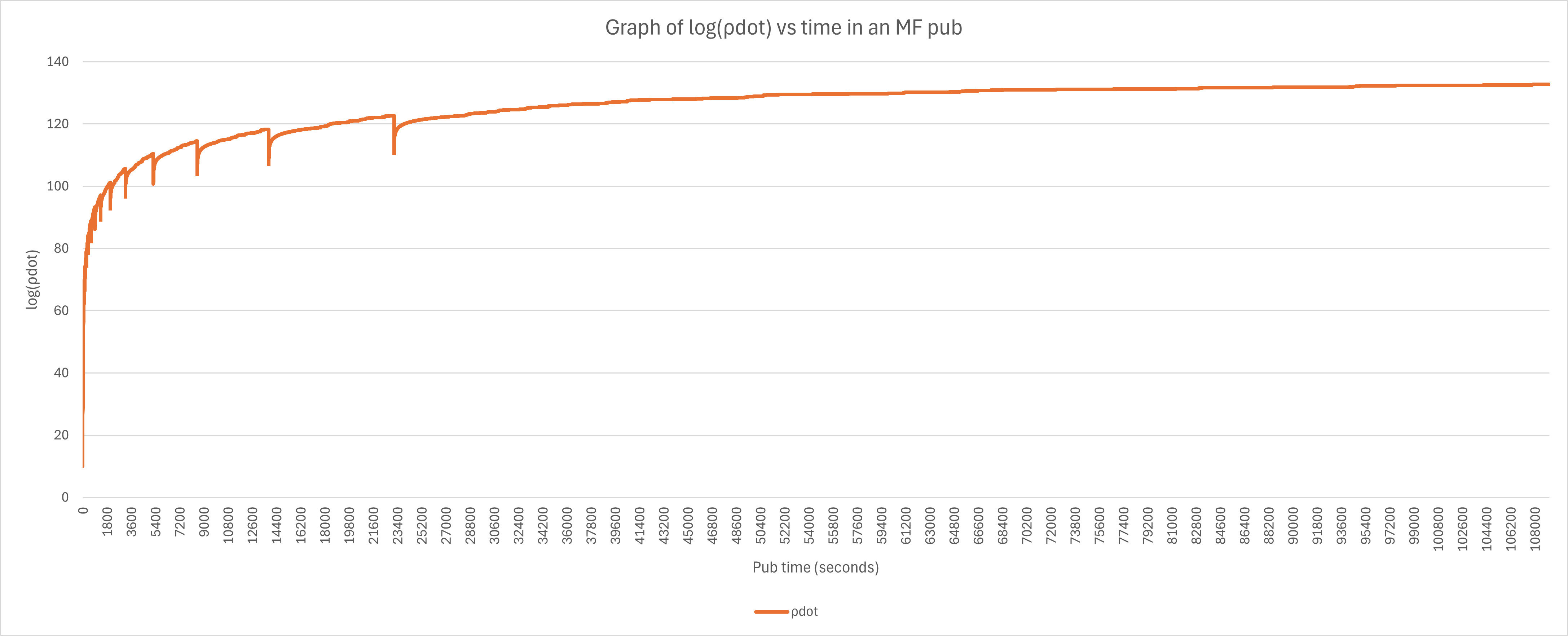
MF is the only custom theory that does not have a strictly positive and the overall theory with the largest spikes in negative . Rates during every publish will NOT be consistently growing. A normal publish looks like this:
There isn’t an exact rule yet on how often you must perform a particle reset. A good baseline is to reset every 1e9 , which is every two levels, but it varies slightly from that. For example, early in the CT you want to reset a bit more often.
It is also important to stop resetting at an appropriate point, you want to only reset once after recovering to your previous publication mark.
We recommend using the sim to check the levels bought with each reset to give you a clearer idea.
For variable buy strats, you can save a bit of time with active buying.
You can also save time by not buying when is very close to its cap () and not buying when is far away from its cap (which typically happens near the end of the CT).
BaP was released on March 10th, 2025, alongside MF. It is based on the Basel Problem, a famous mathematical problem solved by Euler about the convergence of the series , which converges to .
BaP is an idle-friendly custom theory (except for a bit of milestone swapping), and has several similarities with T2.
BaP is much slower than the other CTs early, so it is better to not push it until your other CTs are slow enough. However, BaP holds a secret, a milestone unlocked at e1000 that allows to complete the remaining e200 in under a week! for a total completion time of about 5 months.
is a variable with constant growth once all variables are bought.
The variables work the same way as with T2, the bottom layer has a constant growth, then the growth of each other layer is affected by the value of the layer below, with factors being the variables (except ).
Finally, we have the equation. At the start of the theory, it is the partial sum of the inverse of the squares, which converges. As such, there is no point to buy past a certain point. After getting the first milestone, the equation changes to be the inverse of the remainder of the sum. As we omit more and more of the first terms of the sum, the remainder converges to zero, making useful again. Past earlygame, we approximate .
is also monitored by the exponent, which will always be less than 1, but you will be able to increase it with milestones, and, later, with a variable called .
BaP progress is hard carried by its milestones, which means the best time to publish can vary a lot. For milestones, it is better to push past them to collect the massive boost it gives with all the and you stacked waiting for the milestone. On the contrary, for milestones, it is better to push for them, buy the matching permanent upgrade and publish right away, as you can enjoy the boost right away without waiting for the boost to climb all the way to .
For idle, you autobuy all. For more efficiency, turn off autobuy when your is around x25 away from your publication mark or the next milestone.
BaP active strategies take advantage of active buying. is a unique variable with a low cost scaling and that gains a massive x1024 boost every 64 levels, when ( level) % 64 = 1.
For the strategy, you want to chase those boosts and autobuy when you are close to the next boost (when the cumulative cost of purchases until the boost is below x2 of other variables). When you are not chasing a boost, you can buy at ( level % 64)/2 ratio to other variables.
Milestone Swapping is possible when you don’t have enough milestone points to buy all the milestones. In that case, you can swap between and milestones.
MS is only relevant when you need to stack layers, which typically happens when you unlock a new layer. The cycle goes:
Put the milestone point in the layer wait for and to grow put the milestone point back in the milestone.
You generally want to start a cycle once you buy a new and which boost and respectively.
Like FI, in BaP, you can unlock milestones in 2 ways:
by gaining like normal, or
by purchasing the milestone upgrades for and in the permanent upgrades tab
Buying the milestone upgrades will not give you a milestone, but will instead increase the max level of the milestone that you purchased the upgrade for. For example, if you buy the perma-upgrade for lvl 1, you will permanently unlock the first lvl of the milestone.
While, for most milestones, you unlock the permanent upgrade at the same time you get the milestone point for it, there are 6 exceptions: milestone levels 3,4,5 and milestone levels 4,5,6 in which you unlock the milestone level before you unlock the milestone point, meaning you have a vacant milestone space. This creates an opportunity for milestone swapping between the and milestone, however, in reality, MS is only applicable where you unlock a new milestone level, as, when you unlock a milestone level, it’s generally best to put your milestones into it since you have already built enough , and these MS phases are short anyways.